Calculus Definitions, Theorems, and Formulas

X Facebook Email Copy

Confused about a term in calculus? Check out our explanations for calculus terms. Calculus definitions in simple English! Many of the definitions you’ll find here include videos, graphs and charts to make the explanations easier to understand.

Finding The Calculus Definition You Need

I’ve listed the most popular articles here. Hit Ctrl & F and then type in your search term (or you can just scroll down). Not all articles and definitions are listed here. The best way to find particular calculus definitions is to perform a site search. At the top right of the page (or directly to the right on some browsers), you’ll see a search button. Click on that, and type in the term you want to find.

Calculus Definitions in Alphabetical Order

Click on a term to go to an article and full definition:

Jump to A B C D E F G H I J K L M N O P Q R S T U V W Y-Z

4 Concepts of Calculus

A

B

C

D

E

F

G

H

Calculus Definitions: I to R

I

J

K

Kernel Density Estimation

L

M

N

O

P

Q

R

Calculus Definitions: S to W

S

T

Tangent Line

Tangent Space

U

V

W

X

X-Intercept

Y

Y-Intercept

Z

Compact Spaces

While there are a couple of definitions of compact space, perhaps the easiest way is to understand the concept on the number line. A bounded, closed interval on the real number line is compact; open intervals are not compact.

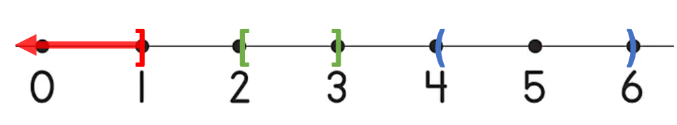
While “compact” might lead you to think “small” in size, this isn’t true in general [1]; Many compact spaces are very large. Basically, compact spaces have stopping points, where you can go no further (think of the closed bracket as a barrier stopping you at 0 on the left and 1 on the right). With non-compact spaces, you can move on until infinity; let’s say you tried to get close to 1 on the open interval (0, 1). You could get within a tenth (0.9) a hundredth (0.99), a thousandth (.999) and so on ad infinitum.

The more precise definition of compactness is not intuitive to grasp: a space is compact if every open cover has a finite subcover. Open covers are collections of open sets that covers a space; in other words, all points of a space is in another member of the collection. Finite subcover refers to the fact that a finite number of these sets can be chosen to also cover the space. Fortunately, you don’t need to dive deep into the depths of topology for most calculus purposes; it’s usually enough to understand that if a space is bounded and closed, then it is compact.

Why is a Compact Spaces Useful?

A compact space is mostly used in the study of functions defined on those spaces. Compactness tends to make a function “well behaved” for analysis.

A compact space acts like a finite space, which allows for making easier proofs. For example, you can often find a minima and maxima in a compact space; on the other hand, is a space is non-compact you have to find suprema and infina instead [2]. Another handy property is that you can define the infinite number line (i.e., the set of all rea numbers) with a finite number of intervals.

Another benefit of compact spaces, and perhaps the most important one in calculus, is that integrals of real-valued, continuous functions on a closed interval [a, b] are always defined because [a, b] is compact.

Compact space: References

[1] Compactness. Retrieved November 3, 2021 from: https://www.msc.uky.edu/droyster/courses/fall99/math4181/classnotes/notes5.pdf
[2] Compactness. Retrieved November 3, 2021 from: math.toronto.edu/ivan/mat327/docs/notes/16-compact.pdf

Euler’s Number

Euler’s number, usually written as e, is a special number with a very important place in mathematics. The first few digits are:

2.7182818284590452353602874713527;

It’s an irrational number, which means you can’t write it as a fraction.

History of Euler’s Number

The number e was “‘discovered” in the 1720s by Leonard Euler as the solution to a problem set by Jacob Bernoulli. He studied it extensively and proved that it was irrational. He was also the first to use the letter e to refer to it, though it is probably coincidental that that was his own last initial.

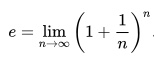
The equation most commonly used to define it was described by Jacob Bernoulli in 1683:

The equation expresses compounding interest as the number of times compounding approaches infinity. With the binomial theorem, he proved this limit we would later call e.

We can actually follow the history of e even further back than Bernoulli. It turns out that e is the base for natural logarithms, and since these were studied extensively by John Napier one hundred years before Euler—in 1614—e is sometimes also called Napier’s constant. Napier published a table of natural logarithms, but didn’t include in his publication the constant they were calculated from.

Ways to Express Euler’s Number

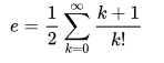
Since Euler’s number is irrational, there is no way to express it as a fraction of integers, or as a finite or periodic decimal number. It comes up so often in both pure and applied math, however, there are many other ways it can be expressed. Some of these include:

In summation notation:

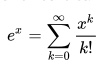
for any real number x, or.

Or using limits:

Or as a sum of trig functions:

Euler’s Number: The First 100 Digits

The first 100 digits of Euler’s number are:

2.7182818284590452353602874713526624977572470936999595749669676277240766303535475945713821785251664274

References

McIntosh, Avery. On Euler’s Number e. Retrieved from http://people.bu.edu/aimcinto/number.e.pdf on May 27, 2018.

O’Connor & Robertson. The Number e. Retrieved from http://www-history.mcs.st-and.ac.uk/HistTopics/e.html on May 27, 2018.

NDT Resource Center. What is e? Retrieved from https://www.nde-ed.org/EducationResources/Math/Math-e.htm on May 27, 2018.

McCartin, Brian J. (2006). “e: The Master of All”. The Mathematical Intelligencer. 28 (2): 10–21 doi:10.1007/bf02987150. Retrieved from https://www.maa.org/sites/default/files/pdf/upload_library/22/Chauvenet/mccartin.pdf on May 27, 2018.

Sandifer, Ed (Feb 2006). “How Euler Did It: Who proved e is Irrational?”. MAA Online. Archived from the original (PDF) on 2014-02-23. Retrieved https://web.archive.org/web/20140223072640/http://vanilla47.com/PDFs/Leonhard%20Euler/How%20Euler%20Did%20It%20by%20Ed%20Sandifer/Who%20proved%20e%20is%20irrational.pdf from May 27, 2018.

What is Propositional Calculus?

Propositional calculus (sometimes called sentential calculus) is a simplified version of symbolic logic; It is a way to analyze truth relationships between compound propositions and their individual parts (Kahn, 2007).

The calculus involves a series of simple statements connected by propositional connectives like:

and (conjunction),
not (negation),
or (disjunction),
if / then / thus (conditional).

You can think of these as being roughly equivalent to basic math operations on numbers (e.g. addition, subtraction, division,…). Only here, instead of numbers, we’re working with propositions (also called statements).

Classical Propositional Calculus

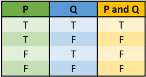
In classical propositional calculus, statements can only take on two values: true or false, but not both at the same time. For example, all of the following are statements:

Albany is the capitol of New York (True),
Bread is made from stone (False),
King Henry VIII had sixteen wives (False).

The following are not propositional statements, because they don’t have a clear true/false answer, or have a subjective answer:

He is a good swimmer,
Banksy is a great artist,
People like bread.

This calculi forms the basis of the majority of logical-mathematical theories; Many complex problems can be reduced to a simple propositional calculus statements, making them easier to solve (Hazelwinkel, 2013). Predicate Calculus is a more complex version, allowing relations, quantifiers, and functions of any number of variables (Goldmakher, 2020).

What is Predicate Calculus?

The object of predicate calculus, a generalization of propositional calculus, is to identify individuals, along with their predicates and properties.
As an example, the following argument cannot be expressed using propositional calculus, but it can be expressed with predicate calculus (ari, n.d.):

All dogs have tails.
Butch is a dog.

From these sentences, you could conclude that Butch (the individual) has a tail. “All dogs have tails” is an example of a predicate—used to describe properties or relationships between individuals or objects. “Dogs” and “Tails” are the terms of the statement, which have the same role in logic as nouns and pronouns in language.

References

Chang, C. & Lee, R. (1997). Symbolic Logic and Mechanical Theorem Proving. New York: Academic Press.
Cundy, H. & Rollett, A. (1989). Mathematical Models, 3rd ed. Stradbroke, England: Tarquin Pub., pp. 254-255.
Goldmakher, L. (2020). Propositional and Predicate Calculus.
Hazelwinkel, M. (2013). Encyclopaedia of Mathematics: Monge—Ampère Equation — Rings and Algebras. Springer.
Kahn, P. (2007). Math 304. Symbolic Logic I: The Propositional Calculus. Retrieved October 29, 2020 from: http://pi.math.cornell.edu/~kahn/SymbLog_PropCalc.pdf
Kari, L/ (n.d.). Predicate Calculus. Retrieved August 4, 2021 from: https://www.csd.uwo.ca/~lkari/logic14.pdf

Sufficiently Large

Loosely speaking, sufficiently large means “large enough” or “sufficiently large numbers”. In mathematics though, we want to define things a little more precisely. Exactly what makes a constant, term or other quantity “large enough” really depends where you’re using the expression. It could be very well defined (for example, a quantity greater than 10) or it could be an estimate. In some cases, it might be theoretically possible but not calculable.

Examples of Sufficiently Large

Weakly complete sequences: A weakly complete sequence is one where every “sufficiently large” natural number is a sum of a sequence’s terms [1]. In other words, it’s a sequence that doesn’t seem to be complete at first, but as you travel down the number line (i.e. as the numbers get “large enough”), the sequence meets the definition of completeness. There are an infinite number of possible sequences; What numbers are sufficiently large depends on the specific sequence.

Hardy-Littlewood conjecture: This famous theory states that every sufficiently large number (i.e. numbers beyond a certain point) can be expressed as a sum of a square and a prime and every large enough number is the sum of a cube and a prime. This theory was later dropped when Hooley [2] & Linnick [3] proved that a sufficiently large enough integer is the sum of two squares and a prime (assuming the extended Riemann hypothesis) [4]. The important thing here is that it happens at some point; the exact numerical value is largely irrelevant.

A Haken-manifold is manifold containing a properly embedded 2-sided incompressible surface; If a 3-manifold meets this property, it’s called sufficiently large [5].

In statistics, we’re often concerned with getting a sufficiently large sample: one that’s big enough to represent some aspect of the population (like the mean, for example). See: Large Enough Sample Condition (StatisticsHowTo.com).

Umbral Calculus

Umbral calculus (also called Blissard Calculus or Symbolic Calculus) is a modern way to do algebra on polynomials. It is a set of exploratory “rules” or a proof technique where indices of polynomial sequences are treated as exponents; Generally speaking, it’s a way to discover and prove combinatorial identities, but it can also be viewed as a theory of polynomials that count combinatorial objects [1].

The name Umbral Calculus was invented by Sylvester, “that great inventor of unsuccessful terminology” [2]. The calculus is based around an umbra, symbol B, which comes from the Latin umbral. Although it is a “shady” way to approach problems, it actually works!

Umbral Calculus Derivation of Bernoulli Numbers

A well known example of umbral notation is the representation of Bernoulli numbers by
(B + 1)² – Bⁿ = 0. After binomial theorem expansion, the B^k is replaced with the B_k to get a recursive formula for the Bernoulli numbers [2]:

The reason why lowering the index “works” has its roots in expressing an infinite sequence of numbers by a transform [2]. In other words, a linear transform B can be defined as
Bxⁿ = B_n.
The “lowering of the index” uses the relationship (X – 1)ⁿ = Xⁿ and adding B to both sides to get B(X – 1)ⁿ = B(Xⁿ).

Development of Umbral Calculus

Umbral calculus is becoming more well known as it heads towards maturity, with applications in several mathematical areas [3]. For example, umbral calculus has been used to solve martingale problems [4] and recurrences as well as counting lattice paths [5].

Despite its simplicity, the early development of umbral calculus was not without its problems. For example, the following “rule” is what Roman & Rota [3] call “baffling” as seemed to imply that a + a ≠ 2:

Umbral Calculus: References

[1] Bucchianico, A. (1998). An introduction to Umbral Calculus. Retrieved May 4, 2021 from: https://www.researchgate.net/publication/2471188_An_introduction_to_Umbral_Calculus
[2] Roman, S. and G.-C. Rota (1978). The umbral calculus. Adv. Math. 27, 95–188.
[3] Ray, N. Universal Constructions in Umbral Calculus. Retrieved May 4, 2021 from: http://www.ma.man.ac.uk/~nige/ucuc.pdfH.
[4] Hammouch, H. (2004). Umbral Calculus, Martingales, and Associated Polynomials. Stochastic Analysis and Applications
Volume 22, Issue 2. pp 443-447.
[5]. Humphreys, K. & Niederhausen, H. (2004). Counting lattice paths taking steps in infinitely many directions under special access restrictions. Theoretical Computer Science 319, 385 – 409

References

[1] Fox, A. & Knapp, M. (2013). A Note on Weakly Complete Sequences. Journal of Integer Sequences.
[2] Hooley, C. (1957). On the representation of a number as the sum of two squares and a prime. Acta, Math. 97, 109-210.
[3] Linnick, J. (1960). An Asymptotic Formula in an Additive Problem of Hardy & Littlewood (Russian). Izv. Akad. Nauk SSR, Ser. Mat. 24. 629-706.
[4] Hardy, G. & Rao, M. Semi r-free and r-free integers; A Unified approach. Canadian Mathematical Bulletin (Sep, 1982).
[5] Waldhausen, F. (1968). On Irreducible 3-Manifolds Which are
Sufficiently Large. Annals of Mathematics, Second Series Volum 87 No. 1. Princeton University.