Numerical integration is a way to find an approximate numerical solution for a definite integral. You use this method when an analytic solution is impossible or infeasible, or when dealing with data from tables (as opposed to functions). In other words, you use it to evaluate integrals which can’t be integrated exactly. The goal of numerical quadrature is to approximate the function accurately with the minimum number of evaluations.
Contents:
Quadrature
For a function of one independent variable (e.g. x), quadraturet replaces the definite integral with a summation, allowing for many “tricky” integration problems, including those with complicated boundaries over higher dimensional spaces, to be integrated. The method is also a building block for the numerical treatment of differential equations.
How Numerical Quadrature Works
Usually, numerical quadrature uses weighted averages to approximate the integral. The general idea is that you replace the definite integral
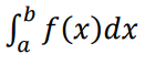
With a weighted sum of a finite number of values from the integrand function
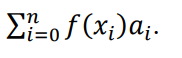
In general, a = x0 and b = xn.
This leads to an approximate answer. How accurate the answer is depends on how many sample points are chosen, and how those contributions are weighted.
Numerical Quadrature Rules
The following numerical quadrature rules are for single intervals:
The trapezoid rule averages the left- and right-hand values from Riemann sums.
Simpson’s rule is an extremely accurate approximation method (probably the most accurate from the Riemann sums options). Instead of rectangles or trapezoids, this numerical quadrature method uses a parabola. A variant is Simpson’s 3/8ths Rule, which uses a slightly different formula.
The Midpoint Rule uses the midpoint of the left-hand and right-hand rectangles.
Open Newton-Cotes formulas are useful when integrand values are given for equally spaced points. In general though, this method is less accurate than other methods (like Gaussian quadrature). The basic steps are:
- Divide a function into equal parts over an interval [a, b],
- Find polynomials that approximate the function (using a technique called Lagrange interpolating polynomials).
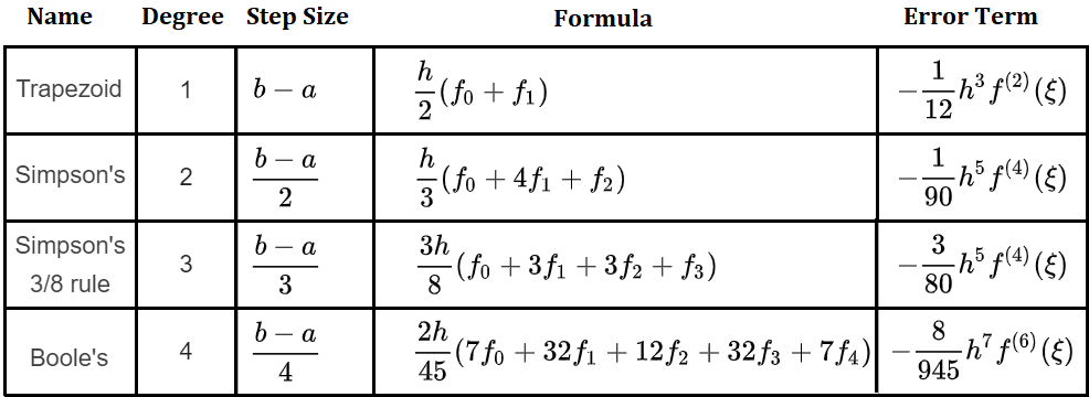
Newton-Cotes formulas can be closed (uses all points) or open (all points except values at the endpoints). The following image shows the closed Newton-Cotes formulas. The degree of accuracy is the largest positive integer that gives and exact value for xk, for every k-value:
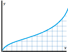
Simple Numerical Integration with Shapes
A very simple form of numerical integration involves using a square grid to find an area. Just superimpose a square grid under a curve, then count the number of squares. If you use relatively small squares, you can get a very good approximation for many functions. If you only need a rough approximation, and aren’t worried about getting an exact answer, this easy method might fit the bill.
Many variations on the basic method exist. For example, you could choose to count full squares only, or approximate the areas of partially filled squares, perhaps counting each partially filled square as one half of a full square.
Riemann Sums, Midpoint, Simpson’s & Trapezoid Rules
Riemann sums (including the midpoint rule, Simpson’s rule, and trapezoid rules) are similar to the “squares” method outlined above, except that they use rectangles instead of squares.
Of this particular set of procedures, Simpson’s rule is quite accurate, and even gives the exact area for any polynomial of third degree or less. For a more detailed explanation of these methods, including step-by-step examples, see the main article on Riemann sums.
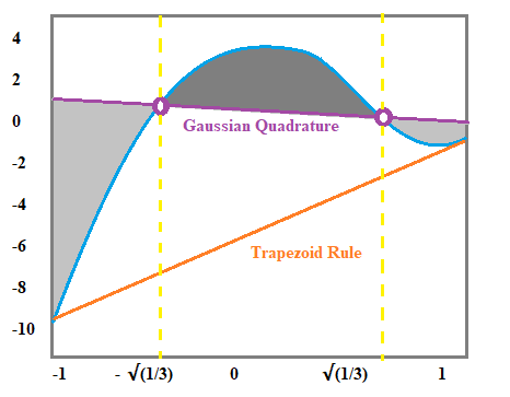
Gaussian Quadrature
Gaussian quadrature gives exact solutions for a polynomial of degree not higher than 2n – 1. The basic idea is that you use a Gaussian curve as the superimposing shape, instead of rectangles or a trapezoid.
Quadrature: References
- Abramowitz, M. and Stegun, I. A. (Eds.). “Integration.” §25.4 in Handbook of Mathematical Functions with Formulas, Graphs, and Mathematical Tables, 9th printing. New York: Dover, pp. 885-887, 1972.
- Corbit, D. “Numerical Integration: From Trapezoids to RMS: Object-Oriented Numerical Integration.” Dr. Dobb’s J., No. 252, 117-120, Oct. 1996.
- Hildebrand, F. B. Introduction to Numerical Analysis. New York: McGraw-Hill, pp. 160-161, 1956.
(2013). Numerical Quadrature. Retrieved January 22, 2020 from: https://www2.math.ethz.ch/education/bachelor/lectures/fs2013/other/nm_pc/Ch07.pdf
Cubature
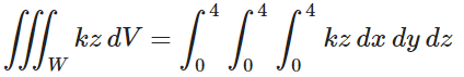
In a general sense of the word, “cubature” is the process for finding the volume of a solid. In calculus, cubature is defined as a numerical computation method for multiple integrals, including those on higher dimensions. For example, on three-dimensional solids or four-dimensional hypercubes, where the limits of integration are vectors. This is in comparison to quadrature, which is numerical computation for a single integral [1].
The basic idea is similar to Riemann sums: The figure is divided into a series of rectangles and finding the limit as these rectangles become thinner. For shapes in higher dimensions (say, over 7), Monte Carlo or similar methods are used [2].
Where to Find Cubature Formula
As you can probably imagine, the number of ways to perform cubature is vast. There are so many in fact, that entire encyclopedias are dedicated to them. Most academic papers on multiple numerical integration refer to one of two books:
- A.H. Stroud. Approximate Calculation of Multiple Integrals, Prentice–Hall, Englewood Cliffs, NJ (1971). This edition is quite comprehensive. Unfortunately, a copy will run you about $500.
- I.P. Mysovskikh. Interpolatory Cubature Formulas, Izdat. Nauka, Moscow, Leningrad (1981). Also a comprehensive book, but the problem is it’s written in the Russian language.
The website Encyclopaedia of Cubature Formulas, developed in Belgium at the Department of Computer Science Katholieke Universiteit Leuven, contains a wealth of cubature tables. For example, you can find formulas here for the cube (including n-cube) and sphere (including n-sphere). Unfortunately, it’s an older site and not very easy to navigate or access (certain parts of the site tell you to login, with no further instructions).
A better solution is to use the formulas found in some statistical software. For example, this R package is for adaptive multivariate integration over hypercubes.
Cubature: References
- Krommer, A. R. and Ueberhuber, C. W. “Construction of Cubature Formulas.” §6.1 in Computational Integration. Philadelphia, PA: SIAM, pp. 155-165, 1998.
- Cubature (Multi-dimensional integration). Retrieved April 8, 2021 from: http://ab-initio.mit.edu/wiki/index.php/Cubature_(Multi-dimensional_integration)