Tangent Line: Definition, Formula & Newton’s Method

Contents:

1. What is a Tangent Line?
   • Horizontal Tangent / How to Find
   • Vertical Tangent / How to Find (opens in new window)
2. Point of Tangency
3. The Tangent Line Problem
4. Finding Tangent Lines: More Examples
5. Newton’s Method
6. Differential Approximation

1. What is a Tangent Line?

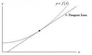
A tangent line is a line that touches a graph at only one point and is practically parallel to the graph at that point. It is the same as the instantaneous rate of change or the derivative .

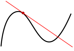
If a line goes through a graph at a point but is not parallel, then it is not a tangent line. This image on the left shows a tangent line at the top left (touching at the red dot). However, the line also crosses the graph at the bottom right (the blue dot); it is not parallel to the graph at that point and therefore it is not a tangent line at that second point.

Horizontal Tangent Lines

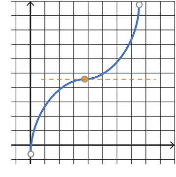
A horizontal tangent line is parallel to the x-axis and shows where a function has a slope of zero. You can find these lines either by looking at a graph (which usually gives an approximation) or by setting an equation to zero to find maximums and minimums.

How to Find Horizontal Tangent Lines

1. From a Graph

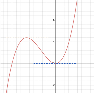
Look for places on a graph where the slope (a.k.a. the derivative) is zero. In other words, look for where the slope is horizontal or flat and parallel to the x-axis. If you have a trace function on your calculator, you should be able to pinpoint the exact coordinates. However, if you have a graph on paper or without that “trace” ability, the position of the horizontal tangent line will usually be an estimate. For example, the graph below appears to have a horizontal tangent at y = 3 (at the graph’s low point). However, the tangent line is actually at y = 3.025:

2. With an Equation

A function or graph has a horizontal tangent line when the first derivative is zero. Another way to think about it: if you find all of the critical points of a differentiable function (i.e. one that has a derivative), a horizontal tangent line occurs wherever there is a relative maximum (a peak) or relative minimum (a low point).

Example question: Find the horizontal tangent line(s) for the function f(x) = x³ + 3x² + 3x – 3.

Step 1: Find the derivative of the function. Using the power rule, the function has a derivative of:
f′(x) = 3x² + 6x – 3

Step 2: Set the derivative equal to zero.
3x² + 6x – 3 = 0.

Step 3: Solve for x:


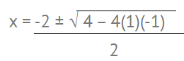
Which simplifies to x = -1 ± √2.

Therefore, the function has two horizontal tangent lines:

• x = -1 + √2.
• x = -1 – √2.

Note that all we’re really doing here is finding critical points.

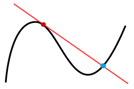
Point of Tangency

The point where the tangent line touches the graph exactly once is called the point of tangency.


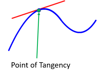
If the tangent line is extended, it may hit the function at another point on the graph, but we’re not concerned about that. What’s important is that the tangent line only skims the graph once at the point of tangency.

The Tangent Line Problem

The tangent line problem: Given a function y = f(x) on an open interval, define the tangent line at a point (x₀, f(x₀)) on the function’s graph.

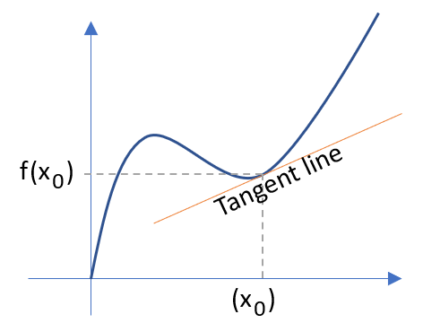
The tangent line problem stumped mathematicians for centuries until Pierre de Fermat and Rene Descartes found a solution in the 17th century; A century later, Newton and Leibniz’s developed the derivative, which approached the tangent line problem using the concept of a limit. The slope of a tangent line is defined as:


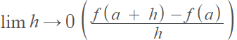
The formula might look complicated, but all you need to do is plug in numbers from a question.

Tangent Line Problem: Example Problems

Example problem #1: What is the tangent line to f(x) = |x| at x = 0?

Step 1: Plug in the “x” value given in the question. This value, given in the question as x = 0, replaces the “a” in the formula:

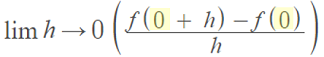
Step 2: Find the function value shown in the top right of the numerator. In other words, we need to find f(0) by plugging in 0 into f(x) = |x|, (which was the function given in the question):

• f(0) = |0| = 0

Step 3: Replace f(0) in the formula with the solution from Step 2:

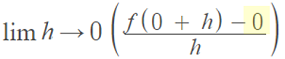
Step 4: Solve the expression at the top left of the numerator, which for this example is f(0 + h). We know from Step 2 that f(0) = 0, so:

• f(0 + h) = 0 + h = h.

Step 5: Insert your value from Step 4 into the formula:

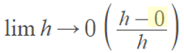
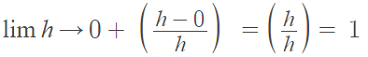
Step 6: Approach the limit from the right:

Step 7: Approach the limit from the left:

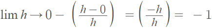
Step 8: Compare Steps 6 and 7. The two-sided limit doesn’t exist because the values are different. In other words, there is not tangent line at to |x| at zero.

Finding the Tangent Line: More Examples

Finding tangent lines for straight graphs is a simple process, but with curved graphs it requires calculus in order to find the derivative of the function, which is the exact same thing as the slope of the tangent line. Once you have the slope of the tangent line, which will be a function of x, you can find the exact slope at specific points along the graph.

Keep in mind that f(x) is also equal to y, and that the slope-intercept formula for a line is y = mx + b where m is equal to the slope, and b is equal to the y intercept of the line.

Example problem: Find the tangent line at a point for f(x) = x².

Note: If you have gone further into calculus, you will recognize the method used here as taking the derivative of the graph. If you know how to take derivatives of a function, you can skip ahead to the asterisked point (*) of step 2.

Step 1: Set up the limit formula. Substituting in the formula x²:

• lim ((x + h)²2 – x²)/h
• h → 0

Step 2: Use algebra to solve the limit formula.

• lim_h→0 (x² + 2xh + h² – x²)/h
• lim_h→0 (2xh + h²)/h
• lim_h→0 h(2x + h)/h
• lim_h→0 2x + h = 2x

This gives the slope of any tangent line on the graph.

Step 3: Substitute in an x value to solve for the tangent line at the specific point.

• At x = 2,
• 2(2) = 4.

That’s it!

What is Newton’s Method?

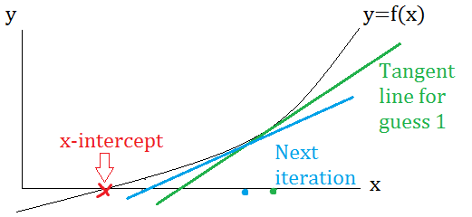
Newton’s method (also called the Newton–Raphson method) is a way to find x-intercepts (roots) of functions. In other words, you want to know where the function crosses the x-axis. The method works well when you can’t use other methods to find zeros of functions, usually because you just don’t have all the information you need to use easier methods. While Newton’s method might look complex, all you’re actually doing is finding a tangent line, then another tangent line, and repeat, until you think you’re close enough to the actual solution.

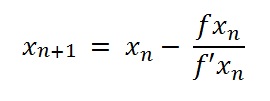
The general form of Newton’s Method is:

If x_n is an approximate solution of f(x) = 0, f′(x)_n ≠ 0, then the next approximate solution is given by:


Where:

• x_n is the x-intercept (initially, your best guess),
• fx_n is the function you’re working with,
• f’x_n is the derivative of the function you’re working with.

What’s basically happening with this equation is each iteration (subsequent calculation) takes you closer and closer to the true solution, as the following image shows. The true solution is marked in red. The blue line is the tangent line for x₀ (Guess 1) and the green line is the tangent line for the second iteration. Eventually, your answers will get closer and closer (converge) to the red x-value.

Newton’s Method: Step by Step Example

Example: Find the x-intercept for f(x) = cos x – x on the interval [0, 2]

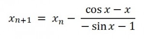
Step 1: Insert your function into the general form of the equation. The bottom half of the equation is the derivative. The derivative of cos x – x is -sin x – 1, so:

Step 2: Take a guess for the actual x-intercept and insert that guess into your function from Step 1. We’re given the interval [0, 2] in the question, so a good guess to start with is 1 (because it’s in the middle of the interval).

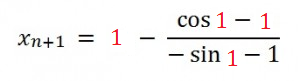
Step 3: Evaluate the function from Step 2 using any calculator (I just used the Google calculator):

• = 1 -( cos(1) -1) / ( – sin(1) – 1))
• = 0.7503638679

Step 4: Repeat Steps 2 and 3, using the new guess for the x-intercept that you obtained from Step 3. This is the second iteration, x₂.
0.7503638679 -( cos(0.7503638679 )-0.7503638679 ) / ( – sin(0.7503638679 ) – 1)) =
0.73911289091

Step 5: Repeat Steps 2 and 3 with your new estimate for as many times as you need. Eventually your answer will converge to a single number. If you compare x₁(Step 2) with x₂ (Step 3), you’ll notice that the first digit is “7” in both cases. That means we’ve got an accuracy of one decimal place. If you perform a third iteration, you’ll have an accuracy to three decimal places (0.739xxxxxxx). Repeat Steps for as many decimal places as you need.

Warning: A downside to Newton’s method; it will not work if you pick a point where the tangent line is horizontal.

Related Articles

• Linearization and Linear Approximation
• Finding the Vertical Tangent

Differential Approximation

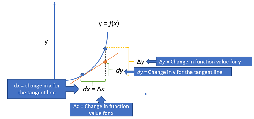
In calculus, differential approximation (also called approximation by differentials) is a way to approximate the value of a function close to a known value. It is just another name for tangent line approximation. In other words, you could say “use the tangent line to approximate a function” or you could say “use differentials to approximate a function“; They mean the same thing.

Differential Approximation Notation

Although tangent line approximation and differential approximation do the same thing, differential approximation uses different notation.

• Δx = change in x,
• Δy = change in y,
• dx = change in x (for the tangent line),
• dy = change in y (for the tangent line).

The image below shows where these pieces fit on a graph.


At first, you may find it a little challenging to see how all of the pieces fit together. But you don’t need to fully understand what they all mean to solve a differential approximation question: the solutions are quite formulaic, and all you really need to know is a couple of different substitutions.
For example, notice on the graph that Δx and dx are of equal lengths. That means you can substitute one expression for the other. The following expressions are also interchangeable:
f(x + Δx) = f(x) + Δy = f(x) + f′(x)Δx.

The next example should make it clear how these substitutions work.

Differential Approximation Example

As a simple example, let’s say the function is f(x) = √(x) and the known value you want to approximate is √(10).

Step 1: Choose a value close to your known value. √(9) is very close to √(10).

Step 2: State Δx (change in the function value for x). Here, we’ve gone from 10 to 9 for our x-value, so Δx = 1.

Step 3: Find the first derivative for the function. For this example, differentiate the function with the power rule (because you can rewrite √(x) as x^½). This gives:

Step 4: Write out the known value as a sum of the function value at x, plus the change in the function value at x:
√(10) = f(x + Δx) ≈ f(x) + f′(x) Δ x (where ′ is prime notation for the derivative. This is where we are using differential approximation instead of the actual value).

Step 5: Substitute in your actual function and derivative:
√(10) = √(x) + Δx

Step 6: Plug in your values, and solve:
√(10) = √(9) + (1)

Giving √(10)= 3.1667, which is close to the actual answer (found with a calculator) of ≈ 3.1623.

References

Desmos graphing calculator.
Department of Mathematics, University of Houston. 1. Differential Approximation (Tangent Line Approximation). Retrieved January 11, 2020 from:
https://online.math.uh.edu/apcalculus/Week03-PracticeProblems-VideoVersion.pdf
Stewart, S. (2009). Study Guide for Stewart’s Single Variable Calculus: Concepts and Contexts, 4th Edition. Cengage Learning.

Morris, J. Section 3.1 – Powers and Polynomials