Gaussian Distribution / Bell Curve Function

Calculus Definitions >

Contents:

1. Gaussian Distribution Definition
2. Gaussian Quadrature
3. Gaussian Function

What is a Gaussian Distribution?

What is a Bell Curve or Gaussian Distribution?

A bell curve is another name for a Gaussian Distribution or normal distribution curve (sometimes just shortened to “normal curve”). The name comes from the fact it looks bell-shaped.

The term “bell curve” is usually used in the social sciences; in statistics, it’s called a normal distribution and in physics, it’s called a Gaussian distribution. However, they all refer to exactly the same thing: a probability distribution that has certain characteristics, including the fact it’s shaped like a bell.

Why the Different Names for the same Distribution?

Although de Moivre first described the normal distribution as an approximation to the binomial, Carl Friedrich Gauss used it in 1809 for the analysis of astronomical data on positions, hence the term Gaussian distribution.

Characteristics of Bell Curves, Normal Curves

1. The arithmetic mean (average) is always in the center of a bell curve or normal curve.
2. A bell curve /Gaussian distribution has only one mode, or peak. Mode here means “peak”; a curve with one peak is unimodal; two peaks is bimodal, and so on.
3. A bell curve has predictable standard deviations that follow the 68 95 99.7 rule (see below).
4. A bell curve is symmetric. Exactly half of data points are to the left of the mean and exactly half are to the right of the mean.

Many phenomena have probability distributions that are bell curves, including:

• Heights
• Weights
• IQ scores
• Growth rates
• Exam scores
• Temperatures connected to Global warming

Bell Curve Standard Deviations

A is a unit of measurement that can help you with figuring out where data items are likely to fall. For example, 68% of all measurements fall within one standard deviation either side of the mean. In other words, the bulk of your data will fall between -1 and +1 standard deviations from the mean. If you go out to two standard deviations, that percentage rises to 95; almost all (99.7%) of your data will fall within three standard deviations.

A Family of Curves

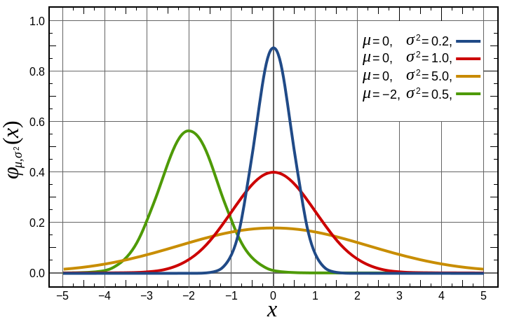
The Gaussian distribution is a continuous family of curves, all shaped like a bell. In other words, there are endless possibilities for the number of possible distributions, given the limitless possibilities for standard deviation measurements (which could be from 0 to infinity). The standard Gaussian distribution has a mean of 0 and a standard deviation of 1. The larger the standard deviation, the flatter the curve. The smaller the standard deviation, the higher the peak of the curve.

What is a Gaussian Distribution Function?

A Gaussian distribution function can be used to describe physical events if the number of events is very large. In simple terms, the Central Limit Theorem (from probability and statistics) says that while you may not be able to predict what one item will do, if you have a whole ton of items, you can predict what they will do as a whole. For example, if you have a jar of gas at a constant temperature, the Gaussian distribution will enable you to figure out the probability that one particle will move at a certain velocity.

• Approximately 68% of events fall within one standard deviation of the mean.
• 95% fall within two standard deviations of the mean.
• 99% fall within three standard deviations from the mean.

What is Gaussian Quadrature?

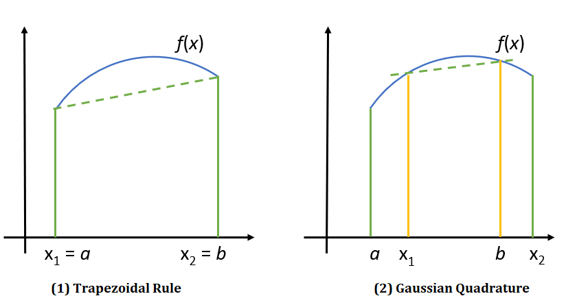
Gaussian quadrature is a way to integrate using weighted sums. The basic idea is that you use a Gaussian curve as the superimposing shape, instead of rectangles or a trapezoid.

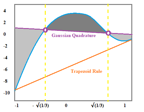
This can lead to better accuracy than other methods, like the trapezoid rule. The optimal nodes (spacings) in Gaussian quadrature are usually uneven.

Gaussian Quadrature Example

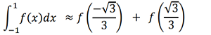
Example question: Perform Gaussian quadrature for = 2 and the interval [, ] = [−1, 1].

Context:
The highest degree of accuracy with Gaussian quadrature is 2n -1. The goal of the procedure is to find values for the integration which achieve this level of accuracy. The formula is exact for functions f(x) = 1, x, x², x³,…, x_n. To integrate a function over the interval of [-1, 1], you need to find x-values (x_i) and weights (w_i) so that:


when f is a polynomial function of degree 2n – 1 = 2(2) − 1 = 3 or less (i.e. a degree of precision 3).

Solution:
Step 1: Integrate for various values of x. We want 2n parameters, so for this example, we’ll integrate the following (2n = 2 * 2 = 4) values:

1. f(x) = 1: w₁ + w₂ = 1 dx = 2
2. f(x) = x: w₁ + w₂ = x dx = 0
3. f(x) = x²: w₁ + w₂ = x² dx = 2/3
4. f(x) = x³: w₁ + w₂ = x³ dx = 1

Solving for ₁, ₂ , w₁ and w₂ gives:

Using Technology

In MATLAB, the Gaussian quadrature rule is implemented with quadl.

Gaussian Function

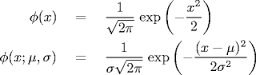
The Gaussian function (named after Carl Friedrich Gauss) is a function that produces the classic bell-shaped curve. It is generally defined as:


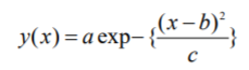
Where:

• exp means “exponential” (i.e. e^x),
• a, b, and c (non-zero) are adjustable constants:
  • a (height of peak),
  • b (position of peak),
  • c (standard deviation or “spread”).

The above formula is used when the constant a is time. The Gaussian can also be specified with a standard deviation (σ or S), where 2 * S * S appears in the denominator of the exponent (Hahn, 1995).

Global Max and Inflection Points

The function has a global maximum (i.e. maximum height) at x = b, where the slope is zero. The following graph shows how manipulating the value for “b” moves the graph along the x-axis:

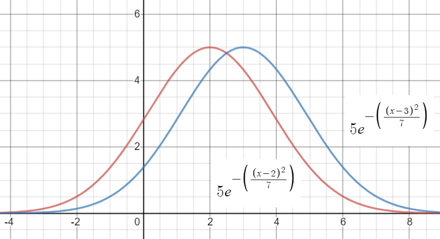
The graph has two inflection points, at x = b ± √(c/2).

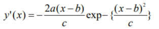
Derivatives

The first derivative of the Gaussian function is:


The second derivative is:

Practical Uses of a Gaussian Function

The Gaussian function has a myriad of uses in mathematics and sciences, including machine learning, physics and biomedical sciences. For example, it is the usual choice for radial basis function (RBF) neural network because it generalizes a global mapping and refines local features without altering the learned mapping (Sundararajan & Lu, 1999). In physics, a Gaussian beam is described by a Gaussian function. The Gaussian is the only function that provides the minimum possible time-bandwidth product along all smooth (analytic) functions (Smith,2020). The Birnbaum-Saunders distribution, used in component lifetime testing, is a mixture of an inverse Gaussian distribution and a reciprocal inverse Gaussian distribution (Shakti, 2022).

References

4.7 Gaussian Quadrature. Retrieved January 13, 2019 from: https://www3.nd.edu/~zxu2/acms40390F15/Lec-4.7.pdf
Abramowitz, M. and Stegun, I. A. (Eds.). Handbook of Mathematical Functions with Formulas, Graphs, and Mathematical Tables, 9th printing. New York: Dover, pp. 887-888, 1972.
Acton, F. S. Numerical Methods That Work, 2nd printing. Washington, DC: Math. Assoc. Amer., p. 103, 1990.
Arfken, G. “Appendix 2: Gaussian Quadrature.” Mathematical Methods for Physicists, 3rd ed. Orlando, FL: Academic Press, pp. 968-974, 1985.
Hahn, L. (1995). The Gaussian Function. Retrieved July 22, 2020 from: http://retina.anatomy.upenn.edu/~rob/lance/gaussian.html
Hildebrand, F. B. Introduction to Numerical Analysis. New York: McGraw-Hill, pp. 319-323, 1956.
Kurzweg, U. (2020). Properties of the Gaussian Function. Retrieved July 22, 2020 from: https://mae.ufl.edu/~uhk/GAUSSIAN-NEW.pdf
Shakti, P. (2022). Birnbaum-Saunders distribution. P-Distribution.com
Smith, J. (2011). Spectral Audio Signal Processing. W3K Publishing.
Stroud, A. H. and Secrest, D. Gaussian Quadrature Formulas. Englewood Cliffs, NJ: Prentice-Hall, 1966.
Sundararajan, N. & Lu, Y. (1999). Radial Basis Function Neural Networks with Sequential Learning. MRAN and Its Applications. World Scientific.

Graph: Desmos.com