Contents (Click to skip to that section):
- What is a Continuous Function?
- Different Types of Continuity
- List of Common Continuous Functions.
- How To Check for The Continuity of a Function.
- Continuous Variables & Data
1. What is a Continuous Function?
Watch the video for an overview and examples, or read on below:
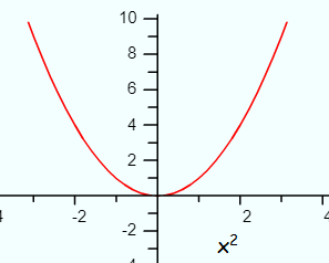
In layman’s terms, a continuous function is one that you can draw without taking your pencil from the paper. If you have holes, jumps, or vertical asymptotes, you will have to lift your pencil up and so do not have a continuous function.
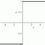
More formally, a function (f) is continuous if, for every point x = a:
- The function is defined at a. In other words, point a is in the domain of f,
- The limit of the function exists at that point, and is equal as x approaches a from both sides,
- The limit of the function, as x approaches a, is the same as the function output (i.e. the y-value) at a.
Order of Continuity: C0, C1, C2 Functions
Order of continuity, or “smoothness” of a function, is determined by how that function behaves on an interval as well as the behavior of derivatives.
C0 Function
A C0 function is a continuous function. More specifically, it is a real-valued function that is continuous on a defined closed interval .
This simple definition forms a building block for higher orders of continuity.
C1 Function
A C1 function is continuous and has a first derivative that is also continuous.
C2 Function
A C2 function has both a continuous first derivative and a continuous second derivative.
Note here that the superscript equals the number of derivatives that are continuous, so the order of continuity is sometimes described as “the number of derivatives that must match.” This is a simple way to look at the order of continuity, but care must be taken if you use that definition as the derivatives must also match in order (first, second, third…) with no gaps. For example, let’s say you have a continuous first derivative and third derivative with a discontinuous second derivative. There are two “matching” continuous derivatives (first and third), but this wouldn’t be a C2 function—it would be a C1 function because of the missing continuity of the second derivative.
Modeling with Order of Continuity
Continuity in engineering and physics are also defined a little more specifically than just simple “continuity.” For example, this EU report of PDE-based geometric modeling techniques describes mathematical models where the C0 surfaces is position, C1 is positional and tangential, and C3 is positional, tangential, and curvature. Which continuity is required depends on the application. For example, modeling a high speed vehicle (i.e. an airplane) needs a high order of continuity compared to a slow vehicle.
2. Different Types of Continuous
If a function is simply “continuous” without any further information given, then you would generally assume that the function is continuous everywhere (i.e. the set of all real numbers from -∞ to + ∞). However, sometimes a particular piece of a function can be continuous, while the rest may not be.
- Continuous on an interval: A function f is continuous on an interval if it is continuous at every point in the interval. For example, you could define your interval to be from -1 to +1. As long as the function is continuous in that little area, then you can say it’s continuous on that specific interval.
- Continuity at an endpoint: There are two possible endpoints for a function: all the way to the left (in the far negative direction), and all the way to the right (in the far positive direction). Assuming the limit exists, “continuity at an endpoint” means that the function is continuous from the right (for the left endpoint) or continuous from the left (for the right endpoint).
Absolutely Continuous
Absolutely continuous real-numbered functions are those functions for which the Fundamental Theorem of Calculus (FTC) holds [1]. In other words, absolute continuity identifies which functions can be antiderivatives: a function on a closed, bounded interval is absolutely continuous on that interval if it is also an antiderivative over that same interval [2].
These functions have the “smoothest” type of continuity, followed by uniform continuity and then plain old continuity. All absolutely continuous functions are continuous, but the converse is not true.
Absolutely continuous functions and random variables are related to each other in the following way: A real-valued random variable X is absolutely continuous if its distribution function FX is absolutely continuous [3]
Formal Definition
The formal definition is frequently used in real analysis, particularly for proving the Fundamental Theorem of Calculus for the Lebesgue Integral [4].
An absolutely continuous function, defined on a closed interval, has the following property. The property is based on a positive number ε and its counterpart, another positive number δ.
- Take the interval for which we want to define absolute continuity, then break it into a set of finite, nonoverlapping intervals. The lengths of these intervals have a sum less than δ,
- Next, consider the absolute values of the differences in the function values at the ends of the intervals; The sum over these intervals is less than ε [5].
In summation notation, we can state the above as: when a finite sequence of non-overlapping intervals satisfies:

then

Where (xk, yk) are the non-overlapping subintervals.
Examples and Properties of Absolutely Continuous Functions
Every convex function and every continuously differentiable function is absolutely continuous [3].
Given a real-valued absolutely continuous function, the following properties hold [6]:
- cf, where c ∈ ℝ
- f + g
- fg
- 1/f, if f(x) ≠ 0 for every x ∈ [a, b]
- |f|.
A few specific examples: The Lipschitz function is absolutely continuous; The Cantor function, is not (although it is continuous everywhere) [7]. The function tan(x) is neither uniformly continuous nor absolutely continuous on the interval [0, π/2].
Absolutely Continuous: References
[1] Heil, C. Real Analysis Lecture notes. 3.5. Abs. cont. and singular functions. Retrieved May 4, 2021 from: https://people.math.gatech.edu/~heil/handouts/ac.pdf
[2] 7.4 Abs. Cont. & Singular Functions. Retrieved May 4, 2021 from: https://www.math.lsu.edu/~rich/Absolute_Continuity
[3] Hill, T. & Berger, A. (2015). An Introduction to Benford’s Law. Princeton University Press.
[4] Pouso, R. (2012). A simple proof of the Fundamental Theorem of Calculus for the Lebesgue integral. Retrieved May 5, 2021 from: https://arxiv.org/pdf/1203.1462.pdf
[5] McGraw-Hill Dictionary of Mathematics, 2/E. (2002). McGraw-Hill.
[6] World Scientific. (2014). Problems and proofs in real analysis. pp. 314-352. Retrieved May 5, 2021 from: https://www.worldscientific.com/doi/10.1142/9789814578516_0013
[7] Real Analysis January 9, 2016 Chapter 6. Differentiation and Integration. Retrieved May 4, 2021 from: https://faculty.etsu.edu/gardnerr/5210/Beamer-Proofs/Proofs-6-5.pdf
Left Continuous Function
A left-continuous function is continuous for all points from only one direction (when approached from the left).
It is a function defined up to a certain point, c, where:
- The function is defined on an closed interval [d, c], lying to the left of c,
- The limit at that point, c, equals the function’s value at that point.
The following image shows a left continuous function up to the point x = 4:
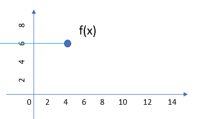
Note how the function value, at x = 4, is equal to the function’s limit as the function approaches the point from the left.
Formal Definition of a Left-Continuous Function
Formally, a left-continuous function f is left-continuous at point c if
limx→c–f(x) = f(c).
In other words, f(x) approaches c from below, or from the left, or for x < c (Morris, 1992). The right-continuous function is defined in the same way (replacing the left hand limit c- with the right hand limit c+ in the subscript).
Right Continuous Function
A right continuous function is defined up to a certain point. The following image shows a right continuous function up to point, x = 4:
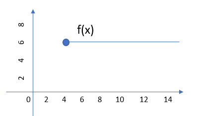
Note that the point in the above image is filled in. On a graph, this tells you that the point is included in the domain of the function. If the point was represented by a hollow circle, then the point is not included in the domain (just every point to the right of it, in this graph) and the function would not be right continuous.
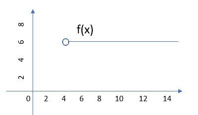
Note that this type of continuity is defined for a point, not for an entire function.
More Formal Definition of a Right Continuous Function
The reason why the function isn’t considered right continuous is because of how these functions are formally defined. Two conditions must be true about the behavior of the function as it leads up to the point:
 exists: The limit of functions must exist at the point. The + sign above the “a” means that the point is being approached from the positive end of the number line; In other words, it’s approaching from the right.
 The right hand limit leading up to the point a, must equal the limit of the function at that point.
In the second example above, the circle was hollowed out, indicating that the point isn’t included in the domain of the function. As the point doesn’t exist, the limit at that point doesn’t exist either.
These Aren’t Really Continuous Functions!
The label “right continuous function” is a little bit of a misnomer, because these are not continuous functions. In order for a function to be continuous, the right hand limit must equal f(a) and the left hand limit must also equal f(a). The definition for a right continuous function mentions nothing about what’s happening on the left side of the point. The function may be continuous there, or it may not be. The only way to know for sure is to also consider the definition of a left continuous function.
Uniformly Continuous Function
A uniformly continuous function on a given set A is continuous at every point on A. The way this is checked is by checking the neighborhoods around every point, defining a small region where the function has to stay inside.
More formally, this is stated as:
A function f : A → ℝ is uniformly continuous on A if, for every number ε > 0, there is a δ > 0; whenever x, y ∈ A and |x − y| < δ it follows that |f(x) − f(y)| < ε.
What that formal definition is basically saying is choose some values for ε, then find a δ that works for all of the x-values in the set. If the same values work, the function meets the definition.
Graph of a Uniformly Continuous Function
Graphically, look for points where a function suddenly increases or decreases curvature. The definition doesn’t allow for these large changes; It’s very unlikely you’ll be able to create a “box” of uniform size that will contain the graph. The function might be continuous, but it isn’t uniformly continuous.
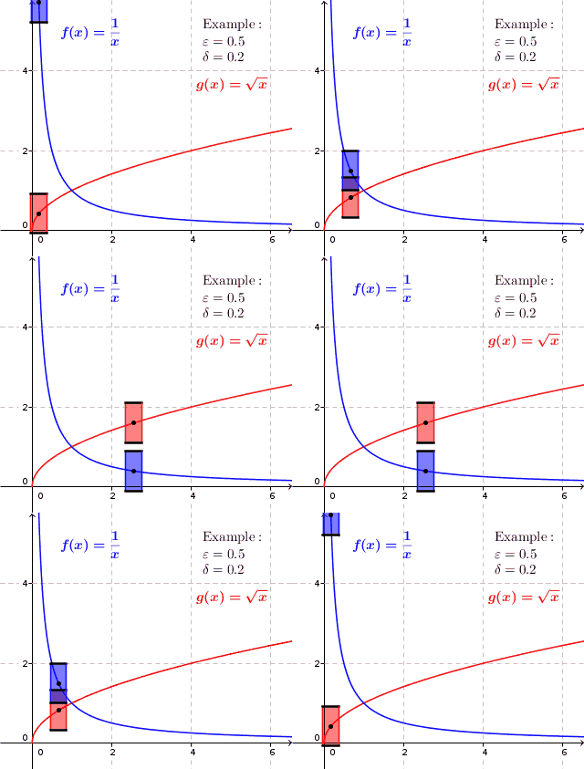
The game here is to try and find a uniform box of height x width = 2ε x 2 δ that, when moved, will keep the graph contained within the edges of the box. So, in a way, the “uniform” part of the definition refers to a “box of uniform size”.
Properties of a Uniformly Continuous Function
These functions share some common properties.
- All of these functions are bounded on a closed interval [a, b] and will achieve a maximum in the set (a, b).
- Every uniformly continuous function is also a continuous function. However, not all continuous functions are uniformly continuous. Therefore, you can think of a these function as ones that are “more” continuous.
- They may or may not be differentiable. Uniform continuity doesn’t necessarily imply differentiability.
3. List of Continuous Functions
All of the following functions are generally continuous:
- Absolute value function,
- Exponential function,
- Logarithmic function,
- All polynomial functions,
- All Power Functions,
- All trigonometric functions.
- The natural exponential function ex (where e is Euler’s number)
5. How to check for the continuity of a function
There are a few general rules you can refer to when trying to determine if your function is continuous. For some functions, you need to do a little detective work. (For a more rigorous approach, see: Continuity Test).
Step 1: Draw the graph with a pencil to check for the continuity of a function. If your pencil stays on the paper from the left to right of the entire graph, without lifting the pencil, your function is continuous. In other words, if your graph has gaps, holes or is a split graph, your graph isn’t continuous.
Step 2: Figure out if your function is listed in the List of Continuous Functions. If it is, then there’s no need to go further; your function is continuous.
Step 3: Check if your function is the sum (addition), difference (subtraction), or product (multiplication) of one of the continuous functions listed in Step 2. If it is, your function is continuous. For example, sin(x) * cos(x) is the product of two continuous functions and so is continuous.
Step 4: Check your function for the possibility of zero as a denominator. The ratio f(x)/g(x) is continuous at all points x where the denominator isn’t zero. In other words, there’s going to be a gap at x = 0, which means your function is not continuous.
That’s it!
Continuous Variables and Data
Contents (Click to skip to that section):
Definition of a Continuous Variable
A continuous variable has an infinite number of potential values.
It’s the opposite of a discrete variable, which can only take on a finite (fixed) number of values.
Watch the video or read on below:
Continuous Variable Range
A continuous variable doesn’t have to include every possible number from negative infinity to positive infinity. In most cases, it’s defined over a range. For example, the range might be between 9 and 10 or 0 to 100. Even though these ranges differ by a factor of 100, they have an infinite number of possible values.
As an example, let’s take the range of 9 to 10. Possible continuous variables include:
- 9, 9.01, 9.001, 9.051, 9.000301, 9.000000801
.
Examples of Continuous Data
A few examples:
- Time it takes you to run the 100 m dash. Watch any timed sporting even and you’ll see times reported to the tiniest hair width. At the time of writing, the world record is held by Usain Bolt, at 9.572 seconds.
- Your weight. Your bathroom scale probably rounds to one tenth of a pound, so you might weight 151.1 lbs. But do you really? You could weight 151.14, or 151.143. The possibilities for weight are endless.
- Money. There was a time in the distant past when money was finite (it was the number of bills and coins in circulation). With the advent of the banking system and cryptocurrency, “money” is now uncountable.
- Car prices. Sure, that Ford might cost you $30k right now. But what about in 100 years? 1,000 years? The price of a car is going to go up and up. You could argue that cars will become obsolete in the future, and therefore there’s a point where car prices will max out. But someone, somewhere is going to have an ancient car worth millions or billions).
What is a Discrete Variable?
A discrete variable can only take on a certain number of values. In other words, they don’t have an infinite number of values. If you can count a set of items, then the variables in that set are discrete variables.
The opposite of a discrete variable is a continuous variable. Continuous variables can take on an infinite number of possibilities.
What is a Discrete Variable? Examples
Some examples of discrete variables:
- Number of quarters in a purse, jar, or bank. Discrete because there can only be a certain number of coins (1, 2, 3, 4, 5…). Coins don’t come in amounts of 2.3 coins or 10 ½ coins, so it isn’t possible for there to be an infinite number of possibilities. In addition, a purse or even a bank is restricted by size so there can only be so many coins.
- The number of cars in a parking lot. A parking lot can only hold a certain number of cars.
- Points on a 10-point rating scale. If you’re graded on a 10-point scale, the only possible values are 1, 2, 3, 4, 5, 6, 7, 8, 9, and 10.
- Ages on birthday cards. Birthday cards only come in years—they don’t come in fractions. So there are a finite amount of possibilities (presumably, about one hundred).
Discrete random variables
Discrete random variables are variables that are a result of a random event. For example, the roll of a die. Discrete random variables are represented by the letter X and have a probability distribution P(X). If you flipped a coin two times and counted the number of tails, that’s a discrete random variable. It’s represented by the letter X. X in this case can only take on one of three possible variables: 0, 1 or 2 [tails].
Continuous Variable Subtype: The Interval Variable & Scale
An interval variable is simply any variable on an interval scale. An interval scale has meaningful intervals between values. The intervals between points on the interval scale are the same. For example, the difference between 10°C and 20°C is the same as the difference between 40°F and 50° F.
An interval variable is a type of continuous variable. Technically (and this is really splitting hairs), the scale is the interval variable, not the variable itself. For example, the variable 102°F is in the interval scale; you wouldn’t actually define “102 degrees” as being an interval variable. That’s because on its own, it’s pretty meaningless.
Problems with Zero
Dates are interval scale variables. For example, a century is 100 years long no matter which time period you’re measuring: 100 years between the 29th and 20th century is the same as 100 years between the 5th and 6th centuries. Although this seems intuitive, dates highlight a significant problem with interval scales: the zero is arbitrary. This means you have to be very careful when interpreting intervals. For example, in the A.D. system, the 0 year doesn’t exist (A.D. starts at year 1). However, some calendars include zero, like the Buddhist and Hindu calendars.
Arbitrary zeros mean that you can’t say that “the 1st millennium is the same length as the 2nd millennium.”
This leads to another issue with zeros in the interval scale: Zero doesn’t mean that something doesn’t exist. For example, just because there isn’t a year zero in the A.D. calendar doesn’t mean that time didn’t exist at that point. To the contrary, it must have, because there are years before 1 A.D. (B.C.!). Similarly, a temperature of zero doesn’t mean that temperature doesn’t exist at that point (it must do, because temperatures drop below freezing).
Arbitrary zeros also means that you can’t calculate ratios. Ratio scales (which have meaningful zeros) don’t have these problems, so that scale is sometimes preferred.
Ratio Variable & Scale

Ratio data this scale has measurable intervals. For example, the difference between a height of six feet and five feet is the same as the interval between two feet and three feet. Where the ratio scale differs from the interval scale is that it also has a meaningful zero. Zero means that something doesn’t exist, or lacks the property being measured. For example, the zero in the Kelvin temperature scale means that the property of temperature does not exist at zero.
Other examples of the ratio scale:
- Age. The clock starts ticking when you are born, but an age of “0” technically means you don’t exist.
- Weight. At 0 pounds, you would weight nothing and therefore wouldn’t exist.
- Height. If you were 0″, you would have no height.
- Sales figures. Sales of zero means that you sold nothing and so sales didn’t exist.
- Quantity purchased. If you bought 0 items, then there were no quantities purchased.
- Time measured from the “Big Bang.”
The Ratio Scale and Negative Numbers
As the “0” in the ratio scale means the complete absence of anything, there are no negative numbers on this scale.
Invariant Under a Similarity Transformation
Data on a ratio scale is invariant under a similarity transformation, y= ax, a >0. For example, you could convert pounds to kilograms with the similarity transformation K = 2.2 P. The ratio stays the same whether you use pounds or kilograms. Although the ratio scale is described as having a “meaningful” zero, it would be more accurate to say that it has a meaningful absence of a property; Zero isn’t actually a measurement of anything—it’s an indication that something doesn’t have the property being measured. For example, 0 pounds means that the item being measured doesn’t have the property of “weight in pounds.”
The Ratio Scale and Ratios
As the name suggests, we can create meaningful ratios between numbers on a ratio scale.
For example, a count of how many tests you took last semester could be zero if you didn’t take any tests. However, if you took two exams this semester and four the last semester, you could say that the frequency of your test taking this semester was half what it was last semester.
Use in Calculus
Scales of measurement, like the ratio scale, are infrequently mentioned in calculus classes. But in applied calculus (a.k.a. in the real world), you likely be using them a lot. For example, economic research using vector calculus is often limited by a measurement scale; only those values forming a ratio scale can form a field (Nermend, 2009).
Next:
Discontinuous Functions
References
Image: By Eskil Simon Kanne Wadsholt – Own work, CC BY-SA 4.0, https://commons.wikimedia.org/w/index.php?curid=50614728
Bogachev, V. (2006). Measure Theory Volume 1. Springer.
Carothers, N. L. Real Analysis. New York: Cambridge University Press, 2000.
Dartmouth University (2005). Continuity. Retrieved December 14, 2018 from: https://math.dartmouth.edu//archive/m3f05/public_html/ionescuslides/Lecture8.pdf
Guha, S. (2018). Computer Graphics Through OpenGL®: From Theory to Experiments. CRC Press.
Kaplan, W. “Limits and Continuity.” §2.4 in Advanced Calculus, 4th ed. Reading, MA: Addison-Wesley, pp. 82-86, 1992.
Larsen, R. Brief Calculus: An Applied Approach.
Morris, C. (1992). Academic Press Dictionary of Science and Technology. Elsevier Science.
Nermend, K. (2009). Vector Calculus in Regional Development Analysis. Comparative Regional Analysis Using the Example of Poland.
Ross, K. (2013). Elementary Analysis: The Theory of Calculus (Undergraduate Texts in Mathematics) 2nd ed. Springer.
Titchmarsh, E. (1964). The theory of functions, 2nd Edition. Oxford University Press.
Tseng, Z. (n.d.). Continuity. Article posted on PennState website. Retrieved December 14, 2018 from: http://www.math.psu.edu/tseng/class/Math140A/Notes-Continuity.pdf