Contents:
Non-Newtonian Calculus
Non-Newtonian calculus, formulated by Robert Katz, Jane Grossman, and Michael Grossman between 1967 and 1972, is a family of non-linear calculi. Classical calculus, primarily developed by Newton and Leibniz in the 17th century, is the “usual” calculus you learn in high school and college. It is linear with additive operators (e.g. derivatives and integrals are both calculated by way of small additions or subtractions). Non-Newtonian calculus is non-linear and doesn’t have additive operators.
After Grossman & Katz’s development of Non-Newtonian calculus, there was a “long period of silence” (Riza & Bugce, 2014) until Bashirov et. al’s 2008 paper Multiplicative calculus and its applications, which appeared in the Journal of Mathematical Analysis and Applications.
Grossman & Katz outlined several branches of Non-Newtonian calculus, including the broad term “multiplicative calculus” and sub-branches of bigeometric calculus and geometric calculus. Other branches, which have largely remained undeveloped, include:
- Anageometric calculus,
- Anaharmonic calculus,
- Anaquadratic calculus,
- Biharmonic calculus,
- Biquadratic calculus,
- Harmonic calculus,
- Quadratic calculus.
Differences Between Classical and Non-Newtonian Calculus
Non-Newtonian calculus has several major differences from classical calculus. For example, exponential calculus (also called geometric calculus in earlier texts) has multiplicative operators. These operators can only be applied to positive functions, so only positive functions are valid in this particular calculus.
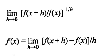
The derivative is defined quite differently as well. In traditional calculus, addition and subtraction are the primary tools to find a derivative. For example, when you find a limit, you’re constantly adding (or subtracting) tiny pieces to approach a particular number. The first non-Newtonian calculus developed, multiplicative calculus, replaces addition and subtraction with division and multiplication. The definition of a derivative changed to focus on a ratio:
Multiplicative Calculus
Multiplicative calculus is a special version of non-Newtonian calculus that uses multiplicative operators. It is built on two basic operations: multiplicative integration and multiplicative derivation. The two operations are inversely related to each other.
Essentially, this type of calculus involves a system in which the addition and subtraction in regular calculus are replaced by multiplication. In the ordinary type of calculus, we base the idea of an integral on an additive rate of change; In this special calculus, we base the idea of an integral on a multiplicative rate of change. There are an infinite number of ways to do this.
Applications of Multiplicative Calculus
Different systems of multiplicative calculi have different applications, but the most widely used systems are geometric calculus and bi-geometric calculus. Geometric calculus is used in biometrical image analysis, as well as to study economic growth, bacterial growth, and radioactive decay. We use bi-geometric calculus to study the theory of elasticity in economics, and it can also help us to understand fractals.
One Example: Geometric Calculus
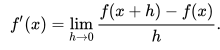
Perhaps the most commonly used multiplicative systems involve geometric calculus. The basis of this is relatively easy to understand, if you understand some basics about derivatives. The regular formula for a derivative is:
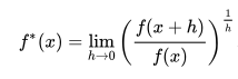
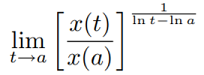
The derivative for geometric calculus— the geometric derivative, we could call it— is:
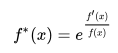
Incidentally, we can write this in terms of our ‘standard derivative’ as:
Interestingly enough, exponential functions are the functions that have a constant derivative in geometric calculus, just as straight lines have a constant derivative in standard classical calculus.
Geometric Calculus
Geometric calculus (also called exponential calculus) is an extension of geometric algebra to include differentiation and integration [1].
Basic Problem of Geometric Calculus and Fundamental Concepts
The basic problem of geometric calculus is as follows:
“Suppose that the value of a positive function h is known at an argument r, and suppose that f, the geometric derivative of h, is continuous and known at each number in [r, s]. Find h(s).” [2]
The solution is:
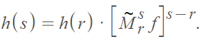
Where the number on the left
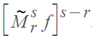
is the geometric integral.
The fundamental concepts of Geometric Calculus are [3]:
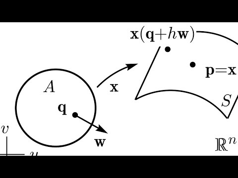
- Coordinate-free differential geometry: Develops concepts on any form or manifold without reference to a particular coordinate system. Although they exist independently of any choice of basis.
- Differentials and codifferentials (which go in the opposite direction from differentials) for mappings and fields.
- Directed integrals (a generalization of the standard Riemannintegral) and differential forms.
- Lie groups (groups that are also differentiable manifolds) as Spin groups. A differentiable manifold is a set on which derivatives and integrals can be calculated.
- Linear and multilinear algebra (tensors, determinants).
- Universal Geometric Algebra – arbitrary dimension and signature.
- Vector derivative and the fundamental theorem of calculus.
- Vector manifolds (for representing any manifold).
Uses of Geometric Calculus
Geometric calculus is challenging to learn and implement; Using it requires some basic knowledge of geometric algebra, an extension of vector algebra. Therefore, you’ll unlikely see it for any general applications. However, the field has brought about several innovations, including Chris Doran and colleagues improvement on general relativity called Gauge Theory Gravity [4, 5].
Geometric Calculus: References
[1] Geometric Calculus. Retrieved July 27, 2021 from: http://geocalc.clas.asu.edu/pdf-preAdobe8/NFMPchapt2.pdf
[2] Grossman, M. & Katz, R. Non-Newtonian Calculus
A Self-contained, Elementary Exposition of the Authors’ Investigations…. Lee Press.
[3] D. Hestenes. Tutorial on Geometric Calculus. Retrieved July 27, 2021 from: http://geocalc.clas.asu.edu/pdf/Tutorial%20on%20Geometric%20Calculus.pdf
[4] C. Doran and A. Lasenby. Geometric Algebra for Physicists. Cambridge: The University Press, 2003.
[5] D. Hestenes, Gauge Theory Gravity with Geometric Calculus, Foundations of Physics 36,
903-970 (2005).
Bigeometric Calculus
“‘So, a standard derivative in [classical] calculus is a limiting quotient of [differences]…So, the idea is: what if you [replace] the differences [with] ratios? At first, when you hear this you think it’s nuts…but I’ve totally bought into this philosophy” ~ Financial engineer Peter Carr [1]
Bigeometric-calculus, developed by Grossman and Katz [2], is a non-Newtonian alternative to the “usual” calculus of Newton and Leibniz; It uses multiplication based differentiation and integration instead of addition. In classical calculus, differences measure changes and sums measure accumulations. In bigeometric calculus, ratios measure changes in arguments and values and products are used for accumulations.
Some authors call the bigeometric calculus the “Volterra calculus”. However, this is not correct: Volterra calculus is not non-Newtonian is quite different from bigeometric calculus [3].
Why Use Bigeometric Calculus?
Bigeometric calculus can be used anywhere problems are exponential in nature. It is particularly suited to problems involving in growth related problems, numerical approximations problems and price elasticity; It has emerged as a useful tool for working with the Black-Scholes model in financial engineering. In some cases involving differential equations, bigeometric calculus has been found to be more accurate than classical calculus [4]. These derivatives also work in the world of fractals, where the ordinary derivative depending on fractal dimension doesn’t exist [5].
Derivatives in Bigeometric Calculus
In Newtonian calculus, linear functions have a constant derivative; In bigeometric calculus, it is the power functions which have a constant derivative. The relationship between the classical and bigeometric derivative (G) is [4]:
![]()
The bigeometric derivative is formally defined as [6]:
Unlike the classical derivative, this derivative is scale invariant (or scale free). In other words, it is invariant for all changes of scale or unit in function arguments and values: if you took a function and doubled it, then compare derivatives for both the doubled and non-doubled functions, they would be the same [3].
References
[1] Tudball, D. (2017). Peter Carr’s Hall of Mirrors. Wilmott. Volume 2017, Issue 89 p. 36-44.
[2] Grossman M., Katz R., (1972), Non-Newtonian Calculus, Lee Press, Piegon Cove, Massachusetts.
[3] Grossman, M. & Katz, R. (2021). Non-Newtonian Calculus. Retrieved May 2, 2021 from: https://sites.google.com/site/nonnewtoniancalculus/-multiplicative-calculus
[4] Boruah, K. & Hazarika, B. (2000). Bigeometric Calculus and its applications. Retrieved May 2, 2021 from: https://arxiv.org/pdf/1608.08088.pdf
[5] Aniszewska, D. & Rybaczuk, M. (2008). Lyapunov type stability and Lyapunov exponent for exemplary multiplicative dynamical systems, Nonlinear Dynamics, Volume 54, Issue 4, Springer, 2008
[6] Filip, & D. Piatecki, C. (2014). An overview on the non-Newtonian calculus and its potential applications to economics. ffhal-00945788
[A] Bashirov, E.M. Kurpınar, and A. Özyapıcı. Multiplicative calculus and its applications.
Journal of Mathematical Analysis and Applications, 337(1):36–48, 2008
[B] Grossman, M. & Katz, R. (1971). Non-Newtonian Calculus. A Self-contained, Elementary Exposition of the Authors’ Investigations. Lee Press.
Riza, M. & Bugce, E. (2014). Bigeometric Calculus and Runge Kutta Method. Retrieved September 19, 2020 from: https://arxiv.org/pdf/1402.2877.pdf
[C] Duff Campbell BA and PhD (1999) Multiplicative Calc and Student Projects, PRIMUS, 9:4, 327-332, DOI: 10.1080/10511979908965938. Retrieved from https://www.tandfonline.com/doi/abs/10.1080/10511979908965938 on April 7, 2019.