What is the Regula-Falsi Method?
The Regula-Falsi method (false position method) is a numerical way to estimate roots of a polynomial. It is a combination of the secant method and bisection methods.
The idea is that if you have a smooth function that doesn’t change much, you can approximate the function with a line using two endpoints [a, b]. The endpoints are joined with a chord; The point where the chord crosses the x-axis is the new “guess” for the root. The appropriate endpoint is updated with the new guess, then the algorithm continues, honing in on the actual root.
The Regula-Falsi tends to be faster than the bisection method and requires fewer iterations, this comes with a higher computational cost. Compared to the secant method, it requires more iterations [1].
How to Use the Regula-Falsi Method
For this example, I’m going to show you the first iteration. The regula-falsi can take a dozen or more iterations to complete, depending on the degree of accuracy you need. The degree of accuracy tells you how close you need to come to the root. For example, within 0.01 or 0.001 (that’s one reason why it’s easier to calculate with software!).
Example Question: Find the root for the continuous function f(x) = x2 + 3x – 5, on the interval [1, 2].
Step 1: Choose an interval so that:
- The function crosses the x-axis and
- f(a) and f(b) have different signs.
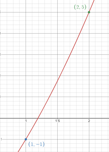
We’re given the closed interval in the question, which is [1, 2]. If you’re not given it then you’ll need to find a reasonable interval around the potential root (try graphing the function to find this interval).
Here is what the function looks like around the root we’re trying to find:

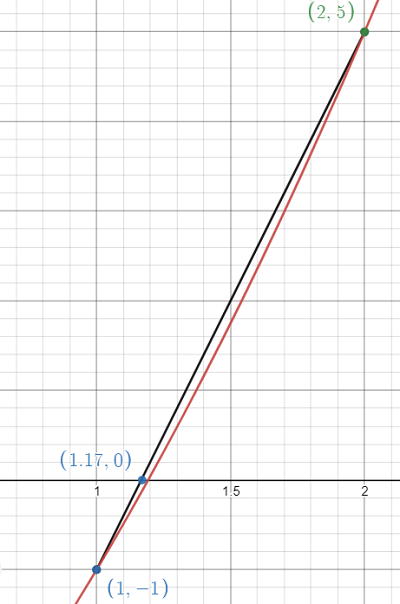
Step 2: Draw a chord (a line segment) between the two function values at a and b and note the position where the chord crosses the x-axis. I used Desmos.com to create the chord:

You can get an accurate location for the point where the chord crosses the x-axis (shown as ≈ 1.17 on the above graph) using a formula:

The formula gives an answer of 1.1667- which we’ll use for the next step.
Step 2: Compute the function value at c:
f(1.1667) = 1.16672 + 3(1.1667) – 5 = -0.14
Step 3: Does f(c) = 0? If so, stop here. You’ve found the root. If not, continue to the next step.
Note: If you’re given a degree of accuracy, then use that instead of zero. For example, if your DOA is 0.01, then the question becomes “Is |f(c)| ≤ 0.01?”
Our function value of -0.14 ≠0, so we’ll continue.
Step 4: Replace a or b with c, depending on the sign of f(c):
- If the sign of f(c) matches the sign of f(a), replace a with c.
- Otherwise, replace b with c.
The sign of f(c) is negative, which matches the sign of f(a), so we’ll replace a with c.
Our new interval is [c, b] = [1.1667, 2].
Step 4: Repeat Steps 2 through 4 until you reach 0 or the desired accuracy.
References
Mahaffy, J. (2010). Solutions of Equations in One Variable. Retrieved July 9, 2021 from: https://jmahaffy.sdsu.edu/courses/s10/math541/lectures/pdf/week03/lecture.pdf