Piecewise Function: Definition, How to Draw

Contents:

1. What is a Piecewise Function?
   • Piecewise Continuous Function
2. Evaluating
3. Graphing by hand
4. Graphing on the TI-89

Definition

A piecewise function is a function made up of different parts. More specifically, it’s a function defined over two or more intervals rather than with one simple equation over the domain. It may or may not be a continuous function.

Piecewise Continuous Function

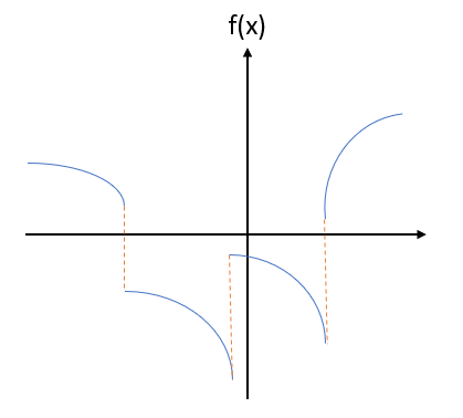
A piecewise continuous function is continuous except for a certain number of points. In other words, the function is made up of a finite number of continuous pieces.

A More Mathematical Definition

A piecewise continuous function f(x), defined on the interval (a < x < b), is continuous at any point x in that interval, except that it could be discontinuous for some finite points x_i (i = 1, 2, 3…) such that a < x_i < b. In addition, both of the following limits exist and are finite (Doshi, 1998):

Examples of a Function that is Not Piecewise Continuous

When trying to figure out if a function is piecewise continuous or not, sometimes it’s easier to spot when a function doesn’t meet the strict definition (rather than trying to prove that it is!).

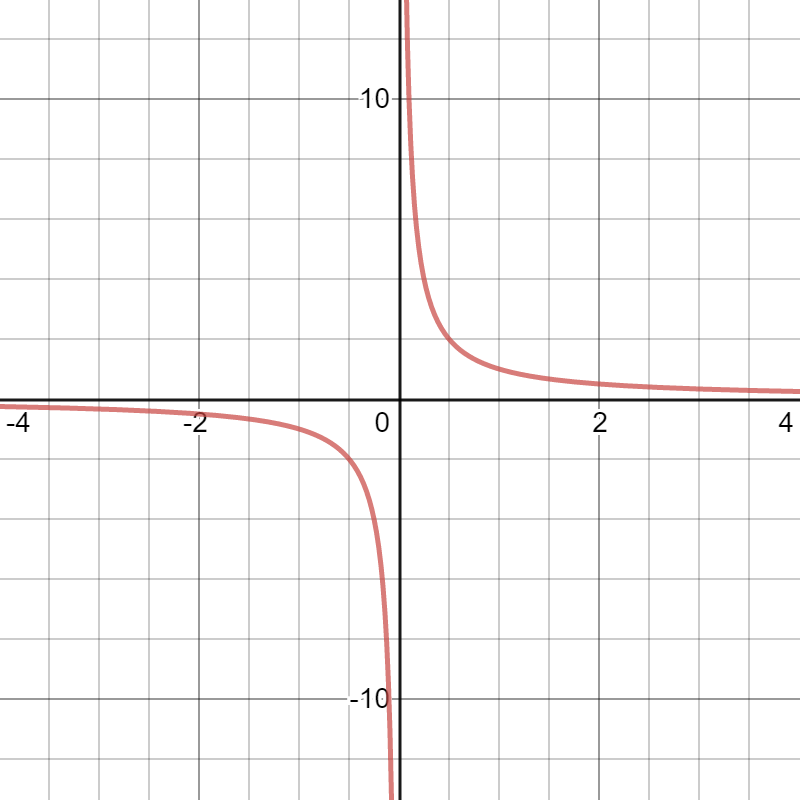
An important part of this definition is that the one-sided limits have to exist. As an example, the function sin(1/x) is not piecewise continuous because the one-sided limit f(0+) doesn’t exist. If a function has a vertical asymptote like this, even at the end of an interval, then it isn’t piecewise continuous.

Perhaps surprisingly, nothing in the definition states that every point has to be defined. A function could be missing, say, a point at x = 0. But as long as it meets all of the other requirements (for example, as long as the graph is continuous between the undefined points), it’s still considered piecewise continuous.

Piecewise Smooth

A piecewise continuous function is piecewise smooth if the derivative is piecewise continuous.

A Caution with Using Graphs to Decide

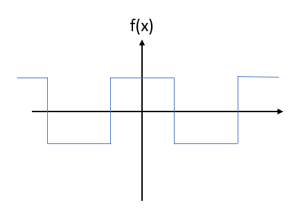
Just because a graph looks like it’s a piecewise continuous function, it doesn’t mean that it is. For example, the square wave function is piecewise, and it certainly looks like a piecewise continuous function. However, the function is not continuous at the integers, so it isn’t an example of this type of function.

Evaluating a Piecewise Function

First identify which piece of your function it belongs in. For example, suppose you wanted to evaluate the following function at x = 0.

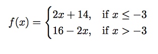
The first thing to note is that this particular function has two pieces, split at x = -3.

If you try to evaluate it by calculating 2x + 14 = 14 (the first piece), you would be wrong. At x = 0, x > – 3, so it is the second part of the piecewise function that applies to your situation. The actual value will be given by 16 – 2x, so:
16 – 2(0) = 16.

This is usually easier to see if you graph the function. A simple procedure is given below.

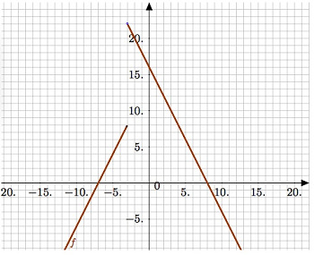
Graphing a Piecewise Function

To graph an piecewise function, first look at the inequalities. For the function above, this would

• x ≤ -3
• x > -3

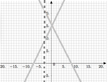
1. On your graph paper, draw vertical dotted lines at each of the values of x listed. In our case, we would be drawing just one line, at x= -3.
2. Draw all the functions given. Draw them very lightly with pencil. You will have two or more functions which may cross; don’t worry about that.
   

   

   
   
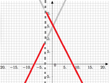
3. Look again at your intervals, and darken/color the graph of your functions only in the relevant intervals: between the vertical lines which mark the changes.
   
4. Finally, erase your light pencil drawing. You now have a neat graph of the piecewise function.

If you graphed


it should look identical to the above.

Piecewise Functions TI 89 “when(” Command

Piecewise functions are functions that are in separate pieces. In other words, instead of one equation to input, you may have several making up one large function. While plotting (and differentiating) piecewise functions by hand can become problematic—especially if you have three or more equations to deal with—the TI89 makes graphing piecewise functions a snap with its “when(“ command.

Piecewise Functions TI 89 “when”: Example

Sample problem: graph the following piecewise functions:

• f(x) = 3x, x is greater than 0,
• f(x) = x + 5, x is less than or equal to 0.

Step 1: Press the HOME key.

Step 2: Press the diamond key and then press F1 to enter the y=editor. Clear any equations in the y=editor by using the arrow keys and pressing the CLEAR key.

Step 3: While you are in the “y1 =” slot, press CATALOG and then press the period “.” (for “W”, which is above the period key). You will immediately be taken to the “when(“ command.

Step 4: Press ENTER to bring the “when(“ command to the “y1 =” slot.

Step 5: While in the “when(“ command, press: x 2nd . 0 , 3 x , x + 5 ) ENTER.
This tells the TI-89 that whenever x is greater than 0, return 3x; whenever x is not greater than 0 (this is the same as whenever x is less than or equal to 0), return x+5

Step 6: Press the diamond key and then press F3 to view the graph.

Note: If you don’t see your graph, check your window settings. Press the diamond key and then press F2 to access the window.

References

Barron & Kastberg. Piecewise Linear Functions. EMT668 Lesson 4. The University of Georgia Department of Mathematics Education
Retrieved from http://jwilson.coe.uga.edu/emt668/EMAT6680.Folders/Barron/unit/Lesson%204/4.html on November 11, 2018
Egbert, Nick. Piecewise Functions. Retrieved from https://www.math.purdue.edu/~egbertn/fa2016/notes/lesson9.pdf on November 11, 2018.
Desmos graphing calculator.Doshi, J. (1998). Analytical Methods in Engineering. Alpha Science Int’l Ltd.
Myint, T. & Debnath, L. (2007). Linear Partial Differential Equations for Scientists and Engineers. Springer Science and Business Media.