Contents:
The Basics
Rules for Derivatives
- Derivative Tables (Quick Reference Guide to Common Derivatives
- Constant Factor Rule
- The Product Rule
- Chain Rule
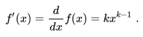
- Functions with exponents (the power rule).
- The Quotient Rule
- Reciprocal Rule: Definition, Examples
- The Sum Rule
Specific Functions
- How to Find the Derivative of Simple Functions:
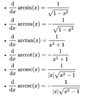
- Inverse Function derivatives.
- Derivative of a Trigonometric Function.
More Definitions & Examples
- Automatic Differentiation
- Continuous Derivative
- Convective Derivative
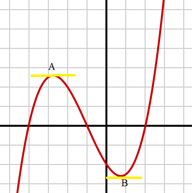
- Critical Numbers
- Derivative Does Not Exist at a Point: 7 Examples
- Left Hand Derivative & Right Hand Derivative
- Differentiate by Parts
- Directional Derivatives
- Epiderivatives
- Explicit Differentiation
- Exterior Derivative
- Faà di Bruno’s Formula: Definition, Example Steps
- Fourth Derivatives
- Fractional Calculus
- Fifth Derivative (Crackle)
- First Derivative Test
- Gateaux Differential
- General Leibniz Rule
- Generalized Derivative: Overview, Examples
- Higher Order Derivatives
- Hukuhara Derivative: Definition
- Implicit Differentiation
- Lanczos Derivative
- Lie Derivative
- Linearity of Differentiation
- Local Derivative
- Logarithmic Derivative
- Mixed Derivative (Partial, Iterated)
- Nth derivative
- Numerical Differentiation
- One Sided Derivative
- Parametric Derivative
- Partial Derivative
- Pi derivative
- Polar Derivative
- Second Derivative Test
- Symmetric Derivative
- Third Derivatives
- Total Differential / Derivative: Formula, Example
- When is a function not differentiable?
- Weak derivatives
What is a Derivative?
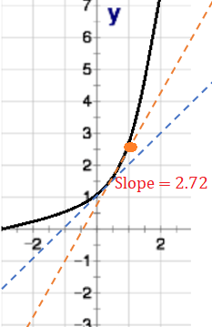
Simply put, it’s the instantaneous rate of change. It tells you how quickly the relationship between your input (x) and output (y) is changing at any exact point in time.
The following formula gives a more precise (i.e. more mathematical) definition.
Limit Definition of a Derivative
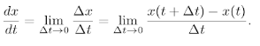
There are short cuts, but when you first start learning calculus you’ll be using the formula.
It’s not uncommon to get to the end of a semester and find that you still really don’t know exactly what one is! That’s because the definition isn’t immediately intuitive; you really get to grasp what one is after you’ve practiced—and practiced. It’s like knowing what an embouchure is in clarinet playing; you can be told that it’s a tongue placement, but it takes many weeks (sometimes months) of practice before you really get a good grasp of the perfect enbouchere and why it’s important.
You can find derivatives in a few different ways. Finding derivatives using the limit definition of a derivative is one way, but it does require some strong algebra skills.
Example problem #1: Find the derivative of f(x) = √(4x + 1)
Step 1: Insert the function into the formula. The function is √(4x + 1), so:
f'(x) = lim Δx → 0 √( 4( x + Δx ) + 1 – √(4x + 1) ) / Δx.
If this looks confusing, all we’ve done is changed “x” in the formula to x + Δx in the first part of the formula.
Step 2: Use algebra to work the formula. Here’s where you’ll benefit from strong algebra skills, because every formula is different.
- Multiply the top and the bottom by √( 4( x + Δx) + 1 + √(4x + 1):
f'(x) = lim Δx → 0 √( 4( x + Δx) + 1 – √(4x + 1) ) * √( 4( x + Δx) + 1 + √(4x + 1) / Δx* √( 4( x + Δx) + 1 + √(4x + 1)
which reduces to:
= lim Δx → 0 4(x + Δx) + 1 – (4x + 1) / Δx(√ (4x + Δx) + 1) + √ 4x + 1 - Distribute the 4:
= lim Δx → 0 (4x + 4Δx + 1 – 4x – 1) / (Δx(√ (4x + Δx) + 1) + √ (4x + 1) - Delete terms. In this case you can delete 4x, Δx and 1.
= lim Δx → 0 4 / ((√ (4x + Δx) + 1) + √ 4x + 1))
Step 3:Take the limit. The Δx will drop out (because it’s an insignificant increment). Again, strong algebra skills will help here:
= 4 / ((√ (4x + 1) + √ 4x + 1)
= 4 / 2 √(4x + 1)
= 2 / √(4x + 1)
That’s it!
Why is The Derivative Important?
Very basically, they are important because they allow you to extract information you didn’t know was there. For example, if you know where an object is (i.e. you have a position function), you can use the derivative to find velocity, acceleration, or jerk (rate of change of acceleration). How? The derivative of…
- …position is velocity.
- …velocity is acceleration.
- …acceleration is jerk.
You can keep on taking derivatives (e.g. fourth, fifth), extracting more and more information from that simple position function. And it doesn’t just work with position; Calculus can work with any function.
What Does Differentiate Mean?
When you differentiate (or “take the derivative”), you’re finding the slope of a function at a particular point. It tells you the rate of change (i.e. how fast or how slow something is changing). For example, if you know the position of a car, you can use differentiation to tell you how fast the car is going at that point.
Let’s say you have a function that models where a car is at any particular point in time. If you differentiate that position function, you end up with a velocity function. In other words, you start with one piece of information (position) and you end up with two pieces of information (position and velocity). In fact, if you know the position function of any object, you can use that to find acceleration and “jerk” as well (jerk is that stomach churning feeling you get when an elevator makes sudden stops and starts). So, differentiating a function allows you to extract a lot of useful information from just a little bit of knowledge.
Slope Formula vs Differentiate Definition
At this point, you may be wondering why you can’t use the slope formula from algebra to find the slope. The answer is: you still can. There’s no difference between finding a slope using the slope formula, or finding the slope using differentiation. The major difference is that differentiation can give you all of the slopes at all of the points, while the slope formula can only give you one at a time. Let’s say you had a thousand coordinate points for the position of a new planet. You can either plug those in a thousand times to the slope formula or you can differentiate once. It’s faster, easier, and a lot less tedious.
Differentiation Definition: Rules
Many rules for differentiation have been formulated. They turn the chore of calculating a zillion slopes or working with the equally tedious limit formulas into relatively quick formulas. You can use the rules to find derivatives quickly for many different types of functions. For example, use the quotient rule if you have two functions being divided, like (x2) / (x + 3x) and use the product rule if they are multiplied together instead.
Sometimes it’s difficult, or impossible to solve an equation for x. For example, complicated functions like 2y2 -cos y = x2 cannot easily be solved for x. In these cases, you’ll have to use a more advanced method called implicit differentiation.
Differentiate Definition References
Anton, H. Calculus: A New Horizon, 6th ed. New York: Wiley, 1999
Beyer, W. H. “Derivatives.” CRC Standard Mathematical Tables, 28th ed. Boca Raton, FL: CRC Press, pp. 229-232, 1987.
TI-89 Derivative Examples
Finding derivatives on the TI 89 or the TI 89 Titanium involves the same steps. That’s because the two calculators are essentially the same, except for a few bells and whistles on the Titanium, like extra memory. These upgrades don’t affect how you find derivatives.
- Derivative TI 89/Titanium Steps
- Evaluate a derivative at a specific value,
- Finding higher derivatives (2nd, 3rd…),
TI 89/Titanium Steps
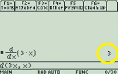
Example problem: Find the derivative of f(x) = 3x.
Step 1: Press F3.
Step 2: Select “1: d( differentiate”. Use the down arrow key or type “1” to select it.
Step 3: Press ENTER.
Step 4: Type in a function, followed by a comma. For example, if your function is 3x then type “3x,”.

Step 5: Type X.
Step 6: Type a closing parenthesis symbol.

Step 7: Press ENTER. The solution (3 in this example) is on the right of the screen.
2. Evaluate a Derivative at a Specific Value
Step 1: Follow Steps 1 through 4 above.
- Press The F3 button
- Select “1: d( differentiate”
- Press ENTER
- Type your function name, followed by a comma.
- Type X
Step 2: Close the parentheses “)”, then type a vertical bar (called the “with” symbol). On the TI-89, you’ll find the “|” key on the left hand side. Don’t press enter yet.
Step 3: Type the value you’re trying to find. For example, type x=3 if you’re trying to find the value of a derivative at x = 3. Press ENTER.
3. Finding Higher Derivatives (2nd, 3rd…)
Example problem: Find the second derivative of f(x) = 3x2 on the TI 89.
Step 1: Follow Steps 1 through 4 in the first section above:
- Press The F3 button
- Select “1: d( differentiate”
- Press ENTER
- Type your function name (3x2), followed by a comma.
- Type X
Step 2: Type a comma, then the number of the derivative you’re trying to find. For this example, you want to find the second derivative, so type “2”. You should have the following syntax:
d(3x^2,x)|x=2
Step 3: Press ENTER.
That’s it! You’re done!
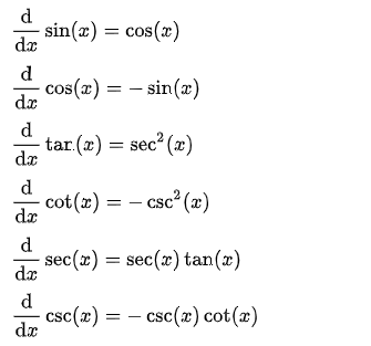
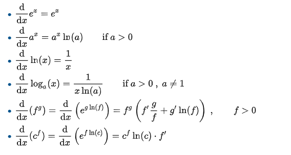
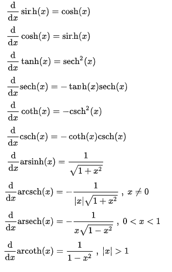
Derivative Tables (Quick Reference Guide to Common Derivatives
Calculus Tables: Contents
- Derivatives:
1. General Rules
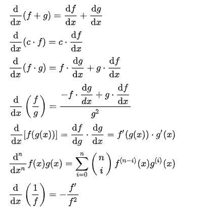
2. Powers and Polynomials
3. Trigonometric Functions
4. Exponential Functions and Logarithmic Functions
5. Inverse Trigonometric Functions
6. Hyperbolic and Inverse Hyperbolic Functions
See: What is a Hyperbolic Function?
References
Wikibooks Tables of Derivatives
Fractional Calculus and the Half Derivative
Watch this 10 minute introduction, or read on below:
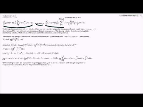
Fractional calculus is when you extend the definition of an nth order derivative (e.g. first derivative, second derivative,…) by allowing n to have a fractional value.
Back in 1695, Leibniz (founder of modern Calculus) received a letter from mathematician L’Hopital, asking about what would happen if the “n” in Dnx/Dxn was 1/2. Leibniz’s response: “It will lead to a paradox, from which one-day useful consequences will be drawn.”
There is no obvious graphical understanding of fractional calculus, and the basic rules we have derived for classical calculus do not all apply—or become very complicated. Simple ideas like the basis for the chain rule or product rule are no longer simple ideas when it comes to this new kind of calculus, and sometimes they just don’t work.
Simple Example of Fractional Calculus: the Derivative of a Power Function
Calculating the derivative of a power function is one of the simplest tasks in calculus, so it is perhaps a good place to begin exploring how a half derivative function might behave.
Let’s define our function of interest, f(x), as:
![]()
Our knowledge of calculus tells us that the first derivative will be
And we can repeat this a times to get the generalized result
Now we know that the factorial is equivalent to the gamma function,
![]()
We can substitute that in in the general formula above, which leaves us with
Now, to find the half derivative, we have to substitute k = 1 and a = ½.
![]()
In the graph below, this half derivative is graphed in purple, alongside the original function (in blue) and the first derivative (in red).
Directional Derivative
The directional derivative tells you the instantaneous rate of change of a function in a particular direction.
You can write this type of derivative as:
![]()
That notation specifies you are looking at the rate of change for the function f(x,y,z) at a specific point (x0, y0, z0). The symbol ∇ is called “nabla” or “del“.
This idea is actually a generalization of the idea of a partial derivative. For a partial derivative, you take the rate of change along one of the coordinate curves while holding all other coordinates constant. For a directional derivative, you must take into account all parts of your directional vector.
Directional Derivative of a Scalar Function
The directional derivative of a scalar function (i.e. a one dimensional function) is relatively easy to define. Along a vector v, it is given by:
![]()
This represents the rate of change of the function f in the direction of the vector v with respect to time, right at the point x.
Properties of the Directional Derivative
There’s one particularly good thing about the directional derivative; many of the properties of the ordinary derivatives hold for it as well.
For example, if our functions f and g are differentiable at a point p:
- The sum rule holds:

- For any constant c, the constant factor rule holds:

- The product rule (otherwise known as Liebniz’s rule) holds:

- And, if g is differentiable at p and h is differentiable at g(p), the chain rule also holds:

What is Automatic Differentiation?
Automatic differentiation (autodiff) uses a computer to calculate derivatives at some specified value, using a mechanical application of the chain rule.
It doesn’t give you a formula, but rather the value of the derivative at the point of interest.
Applications for Automatic Differentiation
Autodiff is used in:
- Data assimilation,
- Design optimization,
- Inverse problems,
- Numerical methods,
- Sensitivity analysis.
It can deal with very complex functions; One of the largest applications was a 1.6 million line code (written in Fortran 77) for research in fluid dynamics.
Advantages
Advantages include:
- It’s efficient and stable,
- Answers are fairly precise,
- It’s generally a good choice if you need to calculate the derivative at a point.
- It’s generally considered a better choice than other computer-based differentiation like finite differencing, symbolic differentiation, or hand coding (Gebremedhin, 2014).
Types of Automatic Differentiation
There are two main types of autodiff:
- Forward mode autodiff,
- Reverse mode autodiff.
Forward mode (also known as director tangent linear mode), is usually used for calculating directional derivatives. It involves finding derivatives of intermediate variables with respect to independent variables. Propagating from one statement to the other is done via the chain rule.
Reverse mode (also known as backward, adjoint or cotangent linear mode) computes the derivatives of dependent variables with respect to intermediate values. Again, propagating from one statement to the next is done according to the chain rule.
These two modes are mathematically equivalent and based on the same principles, but they may require different amounts of time and computer memory.
Automatic Differentiation: References
Bischof, Bucker, Rasch, Slusanschi, and Lang. Automatic Differentiation of the General-Purpose Computational Fluid Dynamics Package. Journal of Fluids Engineering, 2007, volume 129 no 5. pages 652—658. Abstract retrieved from http://fluidsengineering.asmedigitalcollection.asme.org/article.aspx?articleid=1431286 on March 31, 2019Gebremedhin, A. (2014). Research, Automatic Differentiation. Retrieved June 1, 2019 from: https://www.cs.purdue.edu/homes/agebreme/research/coloring-derivatives.html
Bücker, Schiller, Hovland et al. Autodiff. Retrieved from http://www.autodiff.org/?module=Introduction on March 31, 2019.
Grosse, Roger. CSC32 Lecture 10: Automatic Differentiation. The University of Toronto CS. Retrieved from https://www.cs.toronto.edu/~rgrosse/courses/csc321_2018/slides/lec10.pdf on March 30, 2019.
Kourounis, D. et al. (2017). Compile-Time Symbolic Differentiation Using C++Expression Templates. Retrieved June 1, 2019 from: http://arxiv-export-lb.library.cornell.edu/pdf/1705.01729
Wang, Chi-Feng. Automatic Differentiation, Explained. How Do Computers Calculate Derivatives? Retrieved from https://towardsdatascience.com/automatic-differentiation-explained-b4ba8e60c2ad on March 31, 2019.
Epiderivatives
Epiderivatives are derivatives given by epigraphs (the set of points lying on or above a function’s graph) in set-valued optimization problems.
The method unifies the delta and nabla approaches to calculus of variations on time scales (Girejko, et al., 2010).
Epiderivative Definition
Epiderivatives generally fall into the categories of:
- Contingent epiderivatives (introduced by Jahn & Rauh in 1997) or
- Generalized contingent epiderivatives.
The set-valued contingent derivative of a set-valued function H at a certain point is the map with a graph equaling the Bouligand contingent cone of the graph of H at the chosen point (Bigi & Castellani, 2002). More formally, it can be described using notation:
A contingent epiderivative of F at (x, y) is defined as (Rodriguez-Marin et al., 1997):
“…A single-valued map DF (x, y): X → Y whose epigraph coincides with the contingent cone to the epigraph of F at (x, y) i.e. epi (DF (x, y) = T (epi(F), (x, y).”
The generalized contingent epiderivative of F at (x, y) is defined as the following set-valued map:
Dg F (x, y): X → 2Y if
Dg F (x, y) (x) = Min ({y ∈ Y: (x, y) ∈ T (epi(F), (x, y))}).
Higher Order Derivatives
Higher order derivatives are any derivative other than the first (Second, third, fourth, …). The derivative of a function is also a function, so you can keep on taking derivatives until your function becomes f(x) = 0 (at which point, it isn’t possible to take the derivative any more).
Taking the derivative over and over again might seem like a pedantic exercise, but higher order derivatives have many uses, especially in physics and engineering.
Example of Finding Higher Order Derivatives

The first derivative of the function f(x) = x4 – 5x2 + 12x – 13 is:
f′(x) = 4x3 – 10x + 12 (found using the power rule).
But you can differentiate that function again. As you’re differentiating two times, it’s called the second derivative. Using the power rule again, you get: f′′(x) = 12x2 – 10
You can keep on taking the derivative of this particular function five times, when the fifth derivative equals zero. You can’t take a derivative of zero, so you’ll stop there.
Higher Derivatives of the Position Function
Higher order derivatives have many theoretical uses, but they also have a few practical ones. Exactly what kind of information you extract depends upon what kind of function you start with. For example, let’s say you start with a position function.
The first derivative of the position function gives you the velocity function, which gives you the velocity of the object.
The second derivative (of the position function) gives you the object’s acceleration.
The third derivative gives you the jerk— the rate of change of acceleration. It’s called a “jerk” because that’s how a quick change in acceleration feels. Imagine being on a descending elevator that slows down suddenly: that jerking sensation you feel is due to the change acceleration.
The fourth derivative of the position function gives the rate of change of the “jerk”. At this point, the higher order derivatives become more theoretical, but they do have some important uses, especially in safety of high velocity objects (like roller coasters!).
What is the Third Derivative?
The third derivative is the derivative of the second derivative. In other words, it’s the rate of change or slope of the curve of the second derivative.
Jerks and Lurches
The third derivative of the position function is called a jerk, which is the rate of change of acceleration. Let’s suppose that s(t) is an object’s position function:
- The first derivative, s′(t), is the object’s velocity function,
- The second derivative, s′′(t), is its acceleration,
- s′′′(t) is the object’s jerk.
It’s called a jerk (or, less commonly, jolt, lurch, or surge) because changes in acceleration tend to feel “jerky”, especially large ones. A smooth elevator ride feels exactly like that— smooth. But ride on the Tower of Terror, an accelerated drop tower in Disney World’s Hollywood Studios, your stomach will tell you why changes in acceleration are also called “lurches”.
Notation
For any function f(x), f′′′(x) can be defined by several different notations, all of which mean the same thing (from Stewart, 2009):
Example
General steps:
- Take the derivative of the function (using established derivative rules). This is called the first derivative.
- Take the derivative of the new function (i.e. the first derivative). This new function is called the second derivative.
- Take the derivative a third time.
Example : What is the third derivative of f (x) = xn?
Solution, using the power rule multiple times:
- f′(x) = nxn − 1
- f′′′(x) = n(xn − 1)′ = n(n − 1) xn − 2
- f′′′(x) = n(n − 1)(xn − 2)′ = n(n − 1)(n − 2) xn − 3
Fourth and Higher Derivatives
Fourth and higher derivatives are less common. In order to find the fourth derivative, take the derivative another time (i.e. take the derivative of the 3rd derivative). Essentially, you can keep on going on and on to infinity with taking derivatives—it is possible to find the hundredth or thousandth or millionth derivative. However, in reality (and with the types of equations you are likely to encounter), you’ll likely only be able to take derivatives up to the fifth derivative. After that, you’ll probably end up with a constant—and while second, third, and fourth derivatives can give you useful information about a function’s behavior, the hundredth derivative does not.
Sixth Derivative
The sixth derivative (also called pop or pounce) is the result of taking the derivative of a function (usually, the position function) six times. In other words, it’s the derivative of the fifth derivative.
Higher order derivatives, like this one, are rarely seen outside of physics. And when they do occur, they are not usually of much importance. In physics, you would usually find an approximation using a Taylor series, rather than go through the laborious process of finding sixth derivatives. For simple functions, like the one below, finding the sixth derivative is relatively easy. But most real world problems are going to involve functions of greater complexity, which means you’re going to want to approximate the answer with a Taylor series anyway.
Sixth Derivative: Example Problem
Example question: What is the sixth derivative of f(x) = x6 – 3x4 + 9 x – 11?
Solution: Use the power rule and constant rule to take the derivatives six times:
- f′(x) = 6x5 – 12x3 + 9 (First derivative)
- f′′(x) = 30x4 – 36x2 (Second derivative)
- f′′′(x) = 120x3 – 72x (Third derivative)
- f(4) = 360x2 – 72 (Fourth derivative)
- f(5) = 720x (Fifth derivative)
- f(6) = 720 (Sixth derivative)
Snap, Crackle, and Pop
The sixth derivative is called pop after the Snap, Crackle, and Pop of Rice Krispies. J. Codner et al came up with those names (see footnote 17 in Scott et al.) in response to a question asked on the USENET sci.physics newsgroup.
Related Articles
References
Abramowitz, M. and Stegun, I. A. (Eds.). Handbook of Mathematical Functions with Formulas, Graphs, and Mathematical Tables, 9th printing. New York: Dover, p. 11, 1972.
Anton, H. Calculus: A New Horizon, 6th ed. New York: Wiley, 1999
Beyer, W. H. “Derivatives.” CRC Standard Mathematical Tables, 28th ed. Boca Raton, FL: CRC Press, pp. 229-232, 1987.
Bigi, G. & Castellani, M. (2002). K-epiderivatives for set-valued functions and optimization. Mathematical Methods of Operations Research. 401-412.
Girejko, et al., The contingent epiderivative and the calculus of variations on time scales. in Optimization—A Journal of Mathematical Programming and Operations Research. 2010.
Griewank, A. Principles and Techniques of Algorithmic Differentiation. Philadelphia, PA: SIAM, 2000.
Jahn, J. Rauh, R. Contingent epiderivatives and set valued optimization
Math. Methods Oper. Res., 46 (1997), pp. 193-211
Khan, A. et al. (2015). Set-valued Optimization: An Introduction with Applications (Vector Optimization). Springer.
Kimeu, Joseph M., “Fractional Calculus: Definitions and Applications” (2009). Masters Theses & Specialist Projects. Paper 115. digitalcommons.wku.edu/theses/115 Retrieved from https://digitalcommons.wku.edu/cgi/viewcontent.cgi?article=1115&context=theses on April 12, 2018
Kisak, P. (Ed.) (2017). An Overview of Jerk Physics: ” The Meaning of The 3rd Derivative “.
ScienceDirect Fractional Derivatives & Calculus. Retrieved from https://www.sciencedirect.com/topics/physics-and-astronomy/fractional-calculus on April 8, 2019
Rodriguez-Marin, L. & Sama, M. About Contingent Epiderivatives. J. Math. Anal. Appl. 327 (2007). 745-762.
Scott, J. Some Simple Chaotic Jerk Functions in Am. J. Phys., Vol. 65, No. 6, June.
Stewart, J. (2009). Calculus: Concepts and Contexts. Cengage Learning.
Stewart, James. Calculus: Early Transcendentals. Partial Derivatives: Directional Derivs and the Gradient Vector. Retrieved from https://math.libretexts.org/Bookshelves/Calculus/Map%3A_Calculus_-_Early_Transcendentals_(Stewart)/14%3A_Partial_Derivatives/14.6%3A_Directional_Derivatives_and_the_Gradient_Vector on July 27, 2019.
TI89 Users Manual.
Troltzsch , F. Optimal Control and Differential Equations. Maik Nauka/Interperiodica Publishing, 1995.
Viljoen, C & Van der Merwe, L. (1999). Elementary Statistics: Calculations & Interest for Business & Economics. Pearson South Africa.
1. Differential Operator
Contents :
- Differential Operator
- Pseudodifferential Operator
- Total Differential
- Differential Forms
- Schwarzian Derivative
A differential operator tells you to differentiate (take the derivative) with respect to some variable. Typically, the variable differentiated with respect to is x.
Algebraically, the differential operator with respect to x is written as:
d/dx or Dx
The differential operator can also be applied to other variables provided they are a function of x. For example, when y is a function of x, it’s written as:
d/dx(y) = dy/dx
When working with differential operators you use the same rules of differentiation to find the derivative of a function. The simplest differential operator action on a function y gives us the first derivative of the function:
Dy(x) = y′(x)
You can also get the second derivative of the function y(x):
D2y(x) = D(Dy(x)) = Dy′(x) = y′′(x)
Examples: Differential Operator
A typical question will ask you to apply the differential operator to an equation or expression.
Example 1: Apply the differential operator to the expression 5x4
The answer will be the derivative of 5x4 with respect to x. To get the first derivative, just differentiate once, in this case applying the Power Rule:
d/dx (5x4) = 20x4
When you apply the operator to expression 5x4 the answer is 20x4.
Questions may also ask you to apply the differential operator multiple times. These questions are asking you to find higher derivatives.
Example 2: Apply the differential operator twice to y = 5x4
In the first example, applying the operator once resulted in dy/dx = 20x3. To apply it a second time we write:
d/dx (dy/dx) = d/dx (20x3)
The left-hand side of the equation becomes:
d2y/dx2
Apply the Power Rule again to the right-hand side:
d/dx (20x3) = 60x2
Finally, combine the two sides to get the second derivative of y = 5x2
d2y/dx2 = 60x2
2. Pseudodifferential Operator
Pseudodifferential Operators are a generalization of differential operators. This generalization means that every differential operator is a pseudodifferential operator; In other words, pseudodifferentials are obtained by enlarging the class of differential operators. They originated in the latter half of the 20th century at the beginning of elliptic theory, as a natural class of operators which contained the near-inverses of elliptic differential operators.
The inverse of a pseudodifferential operator is also a pseudodifferential operator (Nagy, 2004).
Pseudodifferential Operators Uses
Pseudodifferential operators have a wide variety of applications. They are frequently used:
- In the theory of partial differential equations (PDEs), where many natural objects are pseudodifferentials including the inverse of an elliptic operator,
- In elliptic theory, as a tool on smooth manifolds. They also arise naturally in the classification of elliptic operators and in the reduction of elliptic boundary problems to the boundary,
- Boundary value problems for hyperbolic equations (Treves, 1980),
- Many other practical and theoretical problems in quantum field theory and signal processing.
Representation of Pseudo Differential Operators
The Fourier representation of the operator, represented by p(x, ξ), is:
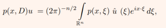
You can think of a differential operator as something that acts on a function as the inverse Fourier transform of a polynomial in the Fourier variable multiplied by the Fourier transform of the function.
Another representation is as a singular integral (Taylor, 2008):
p(x, D)u = ∬ K (x, x – y) u (y) dy,
Where K (x, x – y) = (2π)-n ∬ p (x, Ξ) ei(x – y) · Ξ dΞ
Weyl and Kohn-Nirenberg correspondences
While there are many ways to construct pseudodifferential operators, Weyl and Kohn-Nirenberg correspondences are two of the most popular. In quantum mechanics, these are both examples of “quantization rules” (Heil, 2003).
Recommended Reading
As pseudodifferential operators span an immense field of work, it isn’t possible to delve to deep into their functions in this article. These books give an introduction to pseudodifferential operators and offer many examples of their practical uses:
L. Hormander. “The Analysis of Linear Partial Differential Operators, I,” Second Edition. Springer-Verlag, Berlin (1990).
Volume I is very accessible to newcomers to the field.
E. M. Stein. “Harmonic Analysis: Real-Variable Methods, Orthogonality, and Oscillatory Integrals.” Princeton University Press, Princeton, NJ (1993).
The entire book is devoted to psudodifferentials. Elias M. Stein is the winner of the 2005 Stefan Bergman Prize, American Mathematical Society and the 1998 Wolf Prize for Mathematics, the Wolf Foundation.
M. E. Taylor. “Pseudodifferential Operators.” Princeton University Press, Princeton, NJ (1981).
Main focus is on PDEs.
Logarithmic differentiation
Contents (Click to skip to that section):
- Overview of Logarithmic Differentiation
- When to Use It
- General Evaluation Steps & Simple Example
- Logarithmic Derivative vs. Logarithmic Function
Overview
The logarithmic derivative is where you find the logarithm of a function and then take the derivative. It is often used when it’s easier to find the derivative of the function’s logarithm, rather than the function itself.
One way to define Logarithmic differentiation is where you take the natural logarithm* of both sides before finding the derivative. This can be a useful technique for complicated functions where you can’t easily find the derivative using the usual rules of differentiation.
*The natural logarithm of a number is its logarithm to the base of e.
When to Use Logarithmic Differentiation
In general, functions of the form y = [f(x)]g(x) work best for logarithmic differentiation, where:
- The functions f(x) and g(x) are differentiable functions of x.
- It’s easier to differentiate the natural logarithm rather than the function itself.
The technique can also be used to simplify finding derivatives for complicated functions involving powers, products, and quotients (division).
Although the process sounds simple (and it is, compared to trying to differentiate the “usual” way), it’s really an advanced differentiation technique. You do need to have some knowledge of logarithmic properties and differentiation rules. You should also have some pretty strong algebra skills and be familiar with implicit differentiation.
For example, these logarithm rules will come in handy:
- logb(x · y) = logb(x) + logb(y)
- logb(x / y) = logb(x) – logb(y)
- log(ba) = a log b
General Evaluation Steps & Simple Example
Follow these general steps to find a derivative using logarithmic differentiation:
Step 1: Take the natural log of both sides:
ln y = ln u
Step 2: Use the logarithm rules to remove as many exponents, products, and quotients as possible. In addition, use the following properties of the natural logarithm, if applicable:
- ln (1) = 0,
- ln (e) = 1,
- ln ex = x.
Step 3: Differentiate both sides of the equation.
Step 4: Simplify.
Example question: Differentiate y = xx using logarithmic differentiation:
Step 1: Apply the natural log to both sides:
ln y = ln xx
Step 2: Use the laws to simplify as much as possible:
ln y = ln xx → x ln x
Step 3: Differentiate both sides. For this particular function, use the chain rule on the left side and the product rule on the right:
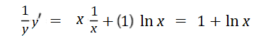
Step 4: Multiply both sides by y:
y′ = y (1 + ln x) = xx(1 + ln x)
A More Complicated Example with the Chain Rule
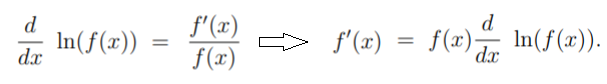
If f is a real-valued function, differentiable and f(x) ≠ 0, then the logarithmic derivative of f is evaluated with the chain rule: f′(x) / f(x). In notation, that’s:
Using similar logic, the log derivative of fg is the log derivative of f + log derivative of g.
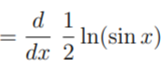
Example problem: Find the logarithmic derivative of ln(√sin x)
Step 1: Convert the radical into an exponent:
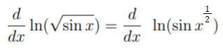
Step 2: Bring the ½ out in front (because of logarithm rule #3, above):
Step 3: Use the chain rule (defined above as lv(f(x))′ = f&prime(x) = f(x)) to get:
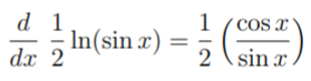
As the cotangent function is the ratio cos(x) / sin(x), this can be rewritten as ½ cot(x).
Complex-Valued Logarithmic Differentiation
The logarithmic derivative becomes more complicated with complex-valued functions. Although you can still use the chain rule f′(z) / f(z).
Example: The logarithmic derivative of an n-degree polynomial function:
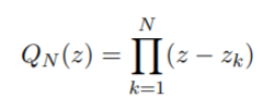
Is given by (Anderson & Eiderman, 2006):
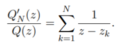
For complex-valued functions like this one, there aren’t actually any logarithms involved (Montgomery, 2014).
Logarithmic Derivative vs. Logarithmic Function
A logarithmic derivative is different from the logarithm function. With logarithmic differentiation, you aren’t actually differentiating the logarithmic function f(x) = ln(x). Instead, you’re applying logarithms to nonlogarithmic functions.
- The logarithm function is a very specific function f(x) = logbx—the inverse of the exponential function.
- The logarithmic derivative can be any function that you find the log for, and take the derivative. For example:
- The digamma function and polygamma functions are the logarithmic derivatives of the gamma function.
- The logarithmic derivative of the sine function is the cotangent function: cotx = (log(sinx))′.
References
Anderson, J. & Eiderman, V. Cauchy transforms of point masses: The log. derivative of polynomials. Annals of Mathematics, 163 (2006), 1057–1076.
Bird, J. (2017). Higher Engineering Mathematics. Routledge.
Ghosh, J. (2004). How to Learn Calculus of One Variable: v. 1. New Age International Publisher.
Larson, R. (2011). Calculus I with Precalculus. Cengage Learning.
Montgomery, H. (2014). Early Fourier Analysis. American Mathematical Society.
Rhode, U et al. (2012). Introduction to Differential Calculus: Systematic Studies with Engineering Applications for Beginners 1st Edition. Wiley.
Partial Derivative
A partial derivative is a derivative where one or more variables is held constant.
When you have a multivariate function with more than one independent variable, like z = f (x, y), both variables x and y can affect z. The partial derivative holds one variable constant, allowing you to investigate how a small change in the second variable affects the function’s output. For example, the partial derivative of z with respect to x holds y constant. Essentially, you find the derivative for just one of the function’s variables.
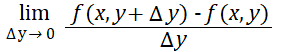
Formally, the partial derivative for a single-valued function z = f(x, y) is defined for z with respect to x (i.e. where y is held constant) as:
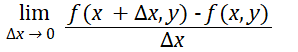
And for z with respect to y (where x is held constant) as:
With univariate functions, there’s only one variable, so the partial derivative and ordinary derivative are conceptually the same (De la Fuente, 2000).
Notation
A partial derivative can be denoted in many different ways.
A common way is to use subscripts to show which variable is being differentiated. For example, Dxi f(x), fxi(x), fi(x) or fx.
Which notation you use depends on the preference of the author, instructor, or the particular field you’re working in. For example, in thermodynamics, (∂z.∂xi)x ≠ xi (with curly d notation) is standard for the partial derivative of a function z = (xi,…, xn) with respect to xi (Sychev, 1991).
How To Find a Partial Derivative: Example
You find partial derivatives in the same way as ordinary derivatives (e.g. with the chain rule or product rule. The only difference is that before you find the derivative for one variable, you must hold the other constant.
Example Question: Find the partial derivative of the following function with respect to x:
f(x, y) = x2 + y4.
Step 1: Change the variable you’re not differentiating to a constant. It doesn’t matter which constant you choose, because all constants have a derivative of zero. For this question, you’re differentiating with respect to x, so I’m going to put an arbitrary “10” in as the constant:
f(x, y) = x2 + 10.
Step 2: Differentiate as usual. For this particular function, use the power rule:
f′x = 2x(2-1) + 0 = 2x.
The partial derivative for this function with respect to x is 2x.
References
Abramowitz, M. and Stegun, I. A. (Eds.). Handbook of Mathematical Functions with Formulas, Graphs, and Mathematical Tables, 9th printing. New York: Dover, pp. 883-885, 1972.
De la Fuente, A. (2000). Mathematical Methods and Models for Economists. Cambridge University Press.
Sychev, V. (1991). The Differential Equations Of Thermodynamics. CRC Press.
Thomas, G. B. and Finney, R. L. §16.8 in Calculus and Analytic Geometry, 9th ed. Reading, MA: Addison-Wesley, 1996.
3. Total Differential
The total differential gives you the total change in a function. For example, let’s say you had a function of two variables:
z = f(x1, x2)
Then dz, the total differential of z, is simply the change in z. Compare that notation to dz/dx, which is the change in z due to the variable x. On its own, “dz” gives you the total change with respect to all of the variables (in this example, x1 and x2).
Note that the total differential can be any variable. For example, dy is the total change in y, and dx is the total change in x. Which variable you use will depend upon which variable you (or someone else) assigned to that function.
Total Differential Formula
The total differential formula uses partial derivatives (∂). Each of the variables in a multivariable function only contributes part of the change in the function. So, the total derivative (which is also called the individual derivative, material derivative, or substantial derivative) is a summation of all of the partial derivatives.
For a function of two variables, z = f(x, y), the total differential of z is:
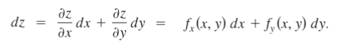
Where dx is the differential of x, and dy is the differential of y. What’s happening in this formula is that to find the total change in y, you’re taking two partial derivatives and adding them together:
- The change in y per unit change in x, multiplied by the change in x,
- The change in y per unit change in y, multiplied by the change in y.
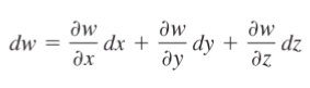
The formula can be extended for more than two variables. For example, the total differential of a three variable function, w = f(x, y, z) is:
Example
Note: As you’re taking a series of partial derivatives here, you may want to read How to Take a Partial Derivative if you’re unfamiliar with the process.
Example question: Find the Total Derivative of y = 99 + 2x1 + 5x2
Solution: Find the partial derivatives of each variable.
- x1: Treat x2 as a constant, and then differentiate. The two constants (99 and x2) have derivatives of zero. The derivative of 2x1 is 2.
- x2: Treat x1 as a constant, and then differentiate. The two constants (99 and x1) have derivatives of zero. The derivative of 5x1 is 5.
Adding the two partial derivatives together gives:
dy = 2 dx1 + 5 dx2
4. Differential Forms
Differential forms are integrands—something (not necessarily a function) that can be integrated “…over a rather complicated domain” (Bachman, 2012, p.1).
Simple Example of a Differential Form
In the expression
x2 is the integrand and x2 dx is the differential form.
What are Differential Forms used for?
When studying differential forms, you’re usually applying them to much more complicated cases than the single variable functions (like x2) you worked with in elementary calculus.
More specifically, differential forms are a special class of tensors where you can find derivatives even in the absence of connections or metrics. You can think of differential forms as a generalization of single variable calculus that works on manifolds, as well as curves, solids, and surfaces.
0-Forms and 1-Forms
A 0-form is simply any function. You dealt with 0-forms in basic calculus.
The general 1-form is:
ω = a dx + b dy.
A fairly simple example of a 1-form is found when working with ordinary differential equations. A 1-form is simply a linear function that acts on a vector and returns a number.
For example, ω(dx, dy)) = dx is a differential form that outputs a number for a set of vectors you input into it.
What Objects do Differential Forms work on?
Differential forms involve dealing with multi-dimensional manifolds, but it’s impossible to visualize what it means to evaluate, say, a 43-form. In fact, anything beyond 3-dimensions is impossible to visualize (even Einstein, who worked with four-dimensions, couldn’t “see” in 4D).
However, it’s possible to understand what’s happening in higher dimensional differential forms (n-forms) if you extend the idea of what happens to the vectors in a 1-form to an n-form. If you evaluate a 1-form, you basically:
- Project onto each coordinate axis, scaling by a constant,
- Adding the results.
The exact same thing happens with n-forms, except you’re dealing with many more vectors.
Schwarzian Derivative
Although it’s called a “derivative”, a Shwarzian isn’t a generalization of the ordinary derivative but rather a differential operator analogous to the ordinary derivative.
The Schwarzian derivative or just “Schwarzian” is, informally speaking, curvature. In complex analysis, it measures how well a Möbius transformation approximates a function. It also gives some other useful information about behavior of functions, especially at critical points [1].
The name is due to Cayley [2], who named the derivative after German mathematician Hermann Schwarz.
Definition of the Schwarzian Derivative
Formally, the Shwarzian is defined as [3]:
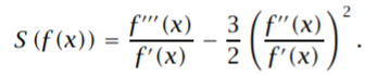
Where:
- f(x) = a real-valued or complex-valued function of one variable,
- f′(x) = first derivative,
- f′′(x) = second derivative,
- f′′′(x) = third derivative.
Critical Points and the Shwarzian
The Schwarzian gives particularly useful information when it is negative. Let’s say x0 is an attracting periodic point of f. A negative Schwarzian tells us one of two things:
- Either the immediate basin of attraction of x0 extends to +∞ or −∞, or
- A critical point of f has an orbit attracted to the orbit of x0.
Möbius Transformations
Möbius transformations (also called fractional linear transformations) are functions of the form:
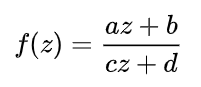
These transformations roughly equate to the constant in an ordinary derivative. Constant functions have ordinary derivatives of zero; In the same way, if a function’s Schwarzian derivative is zero, then that function is a Möbius transformation. Adding a constant to such a function doesn’t change its Schwarzian derivative, nor does multiplying by a constant. With ordinary derivatives, you can pull a constant outside of the function; When you pull a Möbius transformation outside, it just disappears.
Schwarzian Derivative: References
[1] McKinney, W. (2005). The Schwarzian Derivative & the Critical Orbit. Retrieved July 7, 2021 from: https://ocw.mit.edu/courses/mathematics/18-091-mathematical-exposition-spring-2005/lecture-notes/lecture09.pdf
[2] Cayley, A. (1880). On the Schwarzian derivative and the polyhedral functions. Trans. Camb. Phil. Soc., 13.
[3] Ovsienko, V. & Tabachnikov, S. What is the Schwarzian Derivative? Retrieved July 7, 2021 from: https://www.ams.org/notices/200901/tx090100034p.pdf
Differential Operator: References
Andrews, B. Lecture 13.
Arapura, D. (2016). Introduction.
Bachman, D. (2012). A Geometric Approach to Differential Forms. Springer Science & Business Media.
Greub, W. (1972). Connections, Curvature, and Cohomology V1: De Rham cohomology of manifolds and vector bundles. Academic Press.
Heil, C. (2003). Integral Operators, Pseudodifferential Operators, and Gabor Frames. In: Advances in Gabor Analysis, H. G. Feichtinger and T. Strohmer, eds., Birkh¨auser, Boston, 2003, pp. 153–169.
I. C. Gohberg, M. G. Krein Introduction to the theory of linear non-selfadjoint
operators in Hilbert space (Russian), Izdat. Nauka, Moscow, 1965.
Larson, R. & Edwards, B. (2009). Calculus Multivariable. Cengage Learning.
Nagy, G. (2004). Essentials of pseudodifferential operators. Retrieved May 19, 2020 from: https://users.math.msu.edu/users/gnagy/papers/n-pdo.pdf
Taylor, M. (2008). Four Lectures at MSRI. Retrieved May 19, 2020 from: http://mtaylor.web.unc.edu/files/2018/04/msripde.pdf
Treves, J. Introduction to Pseudodifferential and Fourier Integral Operators: Pseudodifferential Operators (University Series in Mathematics). Springer.
Tu, L. (2010). An Introduction to Manifolds. Springer Science & Business Media.