Probability > Maximum Likelihood
What is Maximum Likelihood?
Maximum Likelihood picks parameters of the function under which your data are most likely.
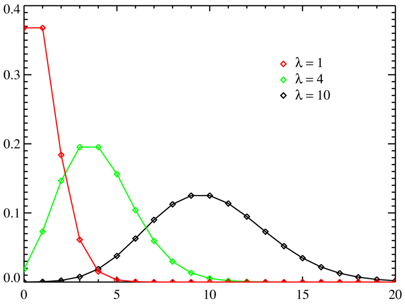
In elementary statistics, you are usually given a model to find probabilities. For example, you might be asked to find the probability that X is greater than 2, given the following Poisson distribution:
X ~ Poisson (2.4)
In this example, you are given the parameter, λ, of 2.4 for the Possion distribution. In real life, you don’t have the luxury of having a model given to you: you’ll have to fit your data to a model. That’s where Maximum Likelihood (MLE) comes in.
MLE takes known probability distributions (such as the normal distribution) and compares data sets to those distributions in order to find a suitable match for the data. A Family of distributions can have an infinite amount of possible parameters. For example, the mean of the normal distribution could be equal to zero, or it could be equal to ten billion and beyond. Maximum Likelihood Estimation is one way to find the parameters of the population that is most likely to have generated the sample being tested. How well the data matches the model is known as “Goodness of Fit.”
- Goodness of fit tests, such as the chi-square test, Kolmogorov–Smirnov test, or BIC, helps you to assess how well a model fits the data. You can also use these tests to compare several models.
- Likelihood is about how plausible a sample is, given your parameter choices.
As a real life example, a researcher might be interested in finding out the mean weight gain of rats eating a particular diet. The researcher is unable to weigh every rat in the population so instead takes a sample. Weight gains of rats tend to follow a normal distribution; Maximum Likelihood Estimation can be used to find the mean and variance of the weight gain in the general population based on this sample.
MLE chooses the model parameters based on the values that maximize the Likelihood Function.
The Likelihood Function
The likelihood of a sample is the probability of getting that sample, given a specified probability distribution model. The likelihood function is a way to express that probability: the parameters that maximize the probability of getting that sample are the Maximum Likelihood Estimators.
Let’s suppose you had a set of random variables X1, X2…Xn taken from an unknown population distribution with parameter Θ. This distribution has a probability density function (PDF) of f(Xi,Θ) where f is the model, Xi is the set of random variables and Θ is the unknown parameter. For the maximum likelihood function you want to know what the most likely value for Θ is, given the set of random variables Xi. The joint probability density function for this example is:
![]()
Finding the maximum likelihood function involves calculus. More specifically, maximizing the PDF. If you aren’t familiar with maximizing functions, you might like this Wolfram Calculator.
In many problems, taking derivatives and setting them to zero is enough to find the MLE. But some models (especially models with constraints or those that have more complicated distributions), the MLE may not exist. In addition, the likelihood function might have local maxima in addition to a global maximum, which complicates finding the “best” parameters.
The Role of the Log-Likelihood in Maximum Likelihood Calculations
To simplify the calculus and reduce numerical underflow issues, it’s usually easier to work with the log-likelihood, because it turns products into sums. For example, if

then the log-likelihood is

Contrast with Bayesian Methods (MAP Estimation)
An alternative is Bayesian parameter estimation, where you have a prior over parameters and compute a posterior. The MAP (Maximum A Posteriori) estimator is then
MAP = arg max [()×()]
Maximum Likelihood Estimator is a special case of MAP when the prior is uniform.
A comparison between MLE and MAP, or a Bayesian approach, is often useful in machine learning contexts.
Next: EM Algorithm.