Contents: (Click to go to that topic)
The integral, along with the derivative, are the two fundamental building blocks of calculus. Put simply, an integral is an area under a curve; This area can be one of two types: definite or indefinite. Definite integrals give a result (a number that represents the area) as opposed to indefinite integrals, which are represented by formulas. Indefinite Integrals (also called antiderivatives) do not have limits/bounds of integration, while definite integrals do have bounds. Watch the video for a quick introduction on to definite integrals, or read on below for more definitions, how-to articles and videos.
Integrals: Definitions
- Additive Interval Property
- Divergent Integrals
- Double Integrals
- Elliptic Integrals
- Isotropic / Anisotropic Definition, Examples
- Fundamental Theorem of Calculus
- Fresnel Integrals
- Fubini’s Theorem
- Gauge Integral
- Improper Integrals
- Integral Bounds / Limits of Integration
- Integral Function
- Integral Kernel
- Integral Operator
- Iterated Integrals
- Lebesgue Integration
- Line Integral
- Mean Value Theorem for Integrals
- Multiple Integrals: Definition, Examples
- Numerical Quadrature (Numerical Integration)
- Order of Integration
- Ordinary Integral
- Probability Integral
- Product Integral
- Quadruple Integral: Definition, Uses of
- Riemann Integral
- Singular Integral: Simple Definition
- Sum Rule
- Stratonovich Integral: Definition
- Triple Integral (Volume Integral)
General How-To Integrals
- Area Between Curve and Y-Axis
- Area Function.
- Indefinite Integrals of power functions
- Constant Rule of Integration
- Finding definite integrals
- Integration Using Long Division: Definition, Examples
- Integration by parts
- Integration by Separation
- Log Rule for Integration
- Integral of a Natural Log
- Integrate with U Substitution
- How to Integrate Y With Respect to X
- Method of Partial Fractions
- Rationalizing Substitutions
- Tabular Integration (The Tabular Method)
- Trig Substitution
Integral Calculus Advanced Problem Solving
- Find Total Distance Traveled (opens in new window)
- How to find the volume of an egg(opens in new window)
- How to prove the volume of a cone(opens in new window)
- How to find the area between two curves
Elliptic Integrals
An elliptic integral is an integral with the form
![]()
Here R is a rational function of its two arguments, w, and x, and these two arguments are related to each other by these conditions:
- w2 is a cubic function or quartic function in x, i.e. w2= f(x) = a0 x4 + a1 x3 + a2 x2 + a3 x + a4
- R(w,x) has at least one odd power of w
- w2 has no repeated roots
In a way, these integrals are generalizations of inverse trigonometric functions. They provide solutions to a wider class of problems than inverse trigonometric functions do; simple problems like calculating the position of a pendulum as well as more complicated problems in electromagnetism and gravitation.
Reducing Elliptic Integrals
As a rule, elliptic integrals can’t be written in terms of elementary functions. There are some special integrals, though: the Legendre elliptic integrals or the canonical elliptic integrals of the first, second and third kinds. Every elliptic integral can be written as a sum of elementary functions and linear combinations of these.
History
These get their name because they were first studied by mathematicians looking to calculate the arc length of an ellipse. The first recorded study of this problem was in 1655 by John Wallis and shortly after by Isaac Newton, who both published an infinite series expansion that gave the arc length of an ellipse. Later, French mathematician Adrien Marie Legendre (who lived between 1752 and 1833) spent nearly forty years researching elliptic integrals, and he was the first to classify elliptic integrals and find ways of defining them in terms of simpler functions.
References
Elliptic Integrals, Elliptic Functions, and Theta Functions. Retrieved from http://www.mhtlab.uwaterloo.ca/courses/me755/web_chap3.pdf on April 22, 2019
Carlson, B. C. NIST Digital Library of Mathematical Functions. Chapter 19: Elliptic Integrals. Release 1.0.22 of 2019-03-15. F. W. J. Olver, A. B. Olde Daalhuis, D. W. Lozier, B. I. Schneider, R. F. Boisvert, C. W. Clark, B. R. Miller, and B. V. Saunders, eds. Retrieved from https://dlmf.nist.gov/19 on April 22, 2019.
Hall, L. (1995). Special Functions. Retrieved May 15, 2019 from: http://web.mst.edu/~lmhall/SPFNS/sfch3.pdf
Jacobi Elliptic functions
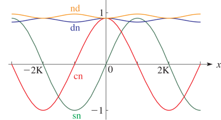
The Jacobi Elliptic functions are a way to express the amplitude φ in terms of an elliptic integral u and modulus k. They share many properties with trigonometric functions and can be thought of as trig function generalizations; In limiting cases where the parameter tends to zero, the Jacobi elliptic functions sn and cn reduce to their trigonometric counterparts: the sine function and cosine function.
They are named after 19th century mathematician Carl Gustav Jacob Jacobi, who contributed to the theory of elliptic functions.
Applications of Jacobi Elliptic Functions
These functions are mostly noted for their historical importance. Practical applications for Jacobi elliptic functions include:
- Descriptions of pendulum motion,
- Design of electronic elliptic filters,
- Solutions for nonlinear ordinary differential equations.
They also appear in various problems of classical dynamics, electrostatics, and hydrodynamics.
Types
There are twelve types of Jacobi elliptic functions denoted by pw(u,k), where:
- u is the real-numbered or complex-numbered argument,
- k is the real or complex modulus (or modular angle, or parameter). Note that convention calls for m if you’re using the parameter or k if you’re using the modulus (which is the square root of m) or modular angle (defined as m = sin2 α),
- p and q can be any of the letters c, s, n or d.
The main types are:
- sn(u, k) = Jacobi elliptic sine function of modulus k, defined as sin φ = sin am(u, k). Analogous to the trigonometric sine function.
- cn(u, k) = Jacobi elliptic cosine function, defined as cos φ = cos am(u, k). Analogous to the trigonometric cosine function.
- tn(u, k) = Jacobi elliptic tangent function: sin φ/cos φ = sn(u, k) / cn (u, k)
- dn (u, k) = difference function (the derivative of φ) =

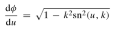
The functions dc, nc, and dc are extensions to imaginary arguments.
Properties of Jacobi Elliptic Functions
Many of these properties follow from properties of trigonometric functions (Lutovac et al., 2001):
- sn2(u, k) + cn(u, k) = 1
- k2sn2(u, k) + dn2(u, k) = 1
- sn(u, k) = sn(-u, k)
- cn(u, k) = cn(-u, k)
- sn(0, k) = 0
- sn(K, k) = 1
- cn(0, k) = 1
- cn(K, k) = 0
References
Lutovac, M. et al., (2001). Filter Design for Signal Processing Using MATLAB and Mathematica. Prentice Hall.
NIST. Digital Library of Mathematical Functions. Retrieved December 3, 2020 from: https://dlmf.nist.gov/22.3#F1
Integral Kernel
An integral kernel is a given (known) function of two variables that appears in an integral equation; This unknown function appears with an integral symbol.
The kernel is symmetric if If K(x, y) = K(y, x).
Notation for the Integral Kernel
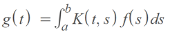
The kernel is denoted by K(x, y):

As well as K(x, y), you might also see slightly different notation depending on what variables are used in the equation. For example:
- A(x, y),
- Ta(x, y), or
- K(x, x′).
What notation is used sometimes depends on exactly what the kernel is representing. Some specific representations include (Wolf, 2013):
- A translation operation a: Ta(x, y),
- Inversions: I0(x, y),
- The operator of differentiation: ∇(x, y).
Avramidi (2015) describes an integral operator on the Hilbert space L2 ([a, b]) as follows:
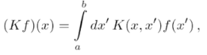
Where the function K(x, x′) is the integral kernel. Note that the author also uses “K” on the left hand side of the equation to denote the operator, a distinction that “…shouldn’t cause any confusion because the meaning of the symbol is usually clear from the context”.
Integral Kernel, or Symbol?
Although the term “integral kernel” is widely used, many authors prefer the alternate term symbol instead, to avoid confusion with many other meanings for the word kernel in mathematics. For example, in geometry, a kernel is the set of points inside a polygon from where the entire boundary of the polygon is visible; In statistics, a kernel is a weighting function used to estimate probability density functions for random variables in kernel density estimation.
Integral Kernel: References
Avramidi, I. (2015). Heat Kernel Method and its Applications 1st ed. Birkhäuser
Paulsen, V. & Raghupathi, M. (2016). An Introduction to the Theory of Reproducing Kernel Hilbert Spaces.
Wolf, K. (2013). Integral Transforms in Science and Engineering. Springer Science & Business Media.
Integral Operator
Generally speaking, an integral operator is an operator that results in integration or finding the area under a curve. It is defined by the integral symbol: ∫.
It’s counterpart in calculus is the differential operator (d/dx), which results in differentiation.
The integral operator is sometimes called a standard integral operator [1] to separate it from special cases used in complex analysis, operator theory and other areas of mathematical analysis.
The term integral operator is also used as a synonym for an integral transform, which is defined via an integral and maps one function to another.
Special Cases of Integral Operator
The first operators appeared at the beginning of the 20th century, at the beginning of the theory of complex-variable functions. Many operators have been developed over the years and are defined very narrowly for special circumstances. They include:
- Alexander integral operator: Defined for a class of analytic functions on the unit disk D [2]:

. - Fredholm operator: Arises in the Fredholm equation, an integral equation where the term containing the kernel function has constants as limits of integration.

- The Volterra integral equation is similar to the Fredholm equation, except that it has variable integral limits.
- A variety of pseudo-differential operators are used to study elliptic differential equations. These operators, as well as Fourier integral operators, make it possible to handle differential operators with variable coefficients in about the same way as differential operators with constant coefficients using Fourier transforms [3].
Integral Operator: References
[1] Anderson, A. SOME CLOSED RANGE INTEGRAL OPERATORS ON SPACES
OF ANALYTIC FUNCTIONS. Retrieved April 23, 2021 from: http://www2.hawaii.edu/~austina/documents/research/aatgpaper2.5.1.pdf
[2] Gao, C. (1992). On the Starlikeness of the Alexander Integral Operator. Proc. Japan Acad. 68. Ser. A.
[3] Hormander, L. Fourier Integral Operators, I. Retrieved April 23, 2021 from: https://projecteuclid.org/journalArticle/Download?urlid=10.1007%2FBF02392052
How to find the area between two curves in integral calculus
Finding the area between two curves in integral calculus is a simple task if you are familiar with the rules of integration (see indefinite integral rules). The easiest way to solve this problem is to find the area under each curve by integration and then subtract one area from the other to find the difference between them. You may be presented with two main problem types. The first is when the limits of integration are given, and the second is where the limits of integration are not given.
Area Between Two Curves: Limits of Integration Given
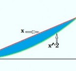
Example problem 1: Find the area between the curves y = x and y = x2 between x = 0 and x = 1.
Step 1: Find the definite integral for each equation over the range x = 0 and x = 1, using the usual integration rules to integrate each term. (see: calculating definite integrals).
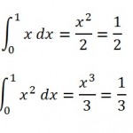
Step 2: Subtract the difference between the areas under the curves. You’ll need to visualize the curves (sketch or graph the curves if you need to); you’ll want to subtract the bottom curve from the top one. The curve on top here is f(x) = x, so:
1⁄2 – 1⁄3 = 1⁄6.
Limits of Integration NOT Given
Example problem: Find the area between the curves y = x and y = x2.
Step 1: Graph the equations. In most cases, the limits of integration will be clear, especially if you’re using a TI-calculator with an Intersection feature (just find the intersections of the two graphs). If you can find the intersection by graphing, skip to Step 3.
Step 2: Find the common solutions of these two equations if you cannot find the intersection by graphing (treat them as simultaneous equations).
Substituting y = x for x in y = x2 gives an equation y = y2, which has only two solutions, 0 and 1.
Putting the values back into y = x to give the corresponding values of x: x = 0 when y = 0, and x = 1 when y = 1. The two points of intersection are (0,0) and (1,1).
Step 3: Complete the steps in Example Problem 1 (limits of integration given) to complete the calculation.
Back to top
Lebesgue Integrals
Lebesgue integrals are a powerful form of integration that can work with the most pathological of functions, including unbounded functions and highly discontinuous functions.
Difference Between Riemann Integration and Lebesgue Integration
Riemann integrals work by subdividing the domain into a number of piecewise constant functions for each sub-interval. Lebesgue integration works by subdividing the range instead. An intuitive example of the difference between the two is given in this analogy by Chapman (2010):
Riemann and Lebesgue add up a group of coins with different face values. Riemann adds up each of the coin’s face values, one by one. Let’s say he picks up a dime, a nickel and then a penny: he’ll count 10 + 5 + 1…. continuing until all of the coins have been added, individually. Then he’ll give his total. In contrast, Lebesgue first sorts the coins into piles of dimes, nickels and pennies. He counts each pile, then sums up the totals from each pile.
When Lebesgue sorts the coins into piles, he’s partitioning the value axis (i.e. the axis with the coin’s numerical values) and taking preimages—sets of function arguments that correspond to a subset in the range. These preimages are the fundamental building blocks of Lebesgue integration.
The basic procedure (Tao, 2010) is:
- Subdivide the function’s range into a finite number of segments.
- Construct a simple function by using a function with values that are the same finitely many numbers.
- Keep on adding points in the range of the original function, taking the limit as you go.
Formal Definition of the Lebesgue Integral
The Lebesgue integral can be formally defined as (Wojas & Krupa, 2017):
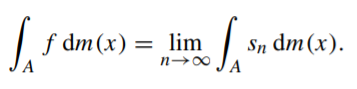
Where:
- sn : A ↦ ℝ is a nondecreasing sequence of nonnegative simple measurable functions, the limit of which is limn→∞ sn(x) = f(x) for every x ∈ A. (note: A is a Lebesgue measurable subset of ℝ).
Note that for this particular definition, the order of sn is not important.
References
Chapman, C. (2010). Real Mathematical Analysis (Undergraduate Texts in Mathematics). Springer New York.
Hunter, J. Riemann Integral. Retrieved January 14, 2019 from: https://www.math.ucdavis.edu/~hunter/m125b/ch1.pdf
Kestelman, H. “Lebesgue Integral of a Non-Negative Function” and “Lebesgue Integrals of Functions Which Are Sometimes Negative.” Chs. 5-6 in Modern Theories of Integration, 2nd rev. ed. New York: Dover, pp. 113-160, 1960.
Papoulis, A. Probability, Random Variables, and Stochastic Processes, 2nd ed. New York: McGraw-Hill, p. 141, 1984.
Tao, T. (2010). 245A, Notes 2: The Lebesgue integral. Retrieved January 14, 2020 from: https://terrytao.wordpress.com/2010/09/19/245a-notes-2-the-lebesgue-integral/
Wojas, W. & Krupa, J. Familiarizing Students with Definition of Lebesgue Integral: Examples of Calculation Directly from Its Definition Using Mathematica. Math.Comput.Sci. (2017) 11:363–381
DOI 10.1007/s11786-017-0321-5
Riemann Integral
The Riemann integral is the classic integral you’re introduced to in introductory calculus classes; Normally shortened to just “integral,” it is found by taking the limit of Riemann sums.
Riemann Integral Overview
The idea behind Riemann integration is that you can find the integral of a bounded, real-valued function by finding the area of small rectangles close to the curve. If the rectangles are below the curve, it’s called the lower sum. Above the curve, it’s called the upper sum.
As these rectangles get smaller and smaller, they approach a limit. This limit will be a very good approximation for the integral, represented by the area under the curve. More specifically, the integral of a function f on interval [a, b] is a real number that can be interpreted geometrically as the signed (±) area under the graph y = f(x) for a ≤ x ≤ b (Hunter, n.d.).
Advantages and Disadvantages of the Riemann Integral
The Riemann integral is relatively simple to define and understand. With Riemann integrals, any continuous function (and many discontinuous functions) can be integrated.
Where Riemann integrals fail is in finding integrals for badly discontinuous or unbounded functions; In those cases, the Riemann integral simply doesn’t exist. This doesn’t mean that the integral doesn’t exist: even the most pathological of functions can be integrated using other methods like Lebesgue integration.
References
Ferreirós, J. “The Riemann Integral.” §5.1.2 in Labyrinth of Thought: A History of Set Theory and Its Role in Modern Mathematics. Basel, Switzerland: Birkhäuser, pp. 150-153, 1999.
Hunter, J. Riemann Integral. Retrieved January 14, 2019 from: https://www.math.ucdavis.edu/~hunter/m125b/ch1.pdf
Jeffreys, H. and Jeffreys, B. S. “Integration: Riemann, Stieltjes.” §1.10 in Methods of Mathematical Physics, 3rd ed. Cambridge, England: Cambridge University Press, pp. 26-36, 1988.
Kestelman, H. “Riemann Integration.” Ch. 2 in Modern Theories of Integration, 2nd ed. New York: Dover, pp. 33-66, 1960.
Integration by Separation
Integration by separation takes a complicated-looking fraction and breaks it down into smaller parts that are easier to integrate.
For example, the following fraction is challenging (impossible?) to integrate using the usual rules of integration:
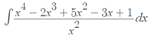
However, you can rewrite it as a series of fractions, using algebra:
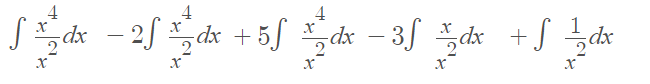
Simplifying, this becomes:
![]()
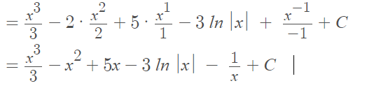
These fractions can be individually integrated, using the power rule and the common integral ∫1⁄xdx = ln |x|:
Trig Substitution
Trig substitution helps you to integrate some types of challenging functions:
- Radicals of polynomial functions, like √(4 – x2),
- Rational powers of the form n/2, e.g. (x2 + 1)(3/2).
Although trig substitution is fairly straightforward, you should use it when more common integration methods (like u substitution) have failed.
The technique is very similar to u substitution: you substitute a new term (one made from integer powers of trig functions) in place of the one you have, in order to make the integration easier. At the end, you simply substitute the original function back in.
Why Is Trig Substitution a Last Resort?
Although it’s straightforward, trig substitution requires you to have a lot of background knowledge. Unlike a table of integrals, you can’t just look up an integral for a particular expression. It’s a must that you are able to recognize the trigonometric identities. Let’s look at an example to see why this is so important.
Example question: Integrate 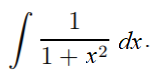
To solve this, you need to consider all of the trig identities to see which would be a good fit. If you aren’t familiar with them, this could be a stumbling block before you’ve even started. In order to solve this particular integral, you need to recognize that it looks very similar to the trig identity
1 + tan2 x = sec2 x.
Here are the solution steps:
Step 1: : Rewrite the expression using a trig substitution (and derivative). The goal here is to get the expression into something you can simplify with a substitution:
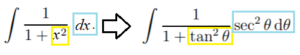
Here, I substituted in tan2θ for x.
As the substitution for x has been made, I also had to change the “dx” to represent the derivative of tan2θ (instead of plain old derivative of “x”). So the new “dx” became sec2 θ dθ.
Step 2: : Simplify by using a trig identity. In this example, we’ve been heading towards changing 1 + tan2 x to sec2 x. There’s no magic here—if you chose the correct trig function in Step 1, you should already know which trig identity you’re going to use here:
![]()
Step 3: : Simplify using algebra (if possible). For this example, notice that we can cancel out the sec2 in the numerator and denominator,
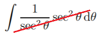
leaving just
∫ 1 dθ.
Step 4: Integrate. The integral of a constant function is just the constant * x (or constant * θ) + C, so:
∫ 1 dθ = θ + C
Step 5: Substitute your original term back in. In Step 1, I substituted tan-1 θ for x, so putting that back in gives the solution:
= tan -1 x + C
Useful Background Information
As you may be able to tell from the above example, trig substitution requires you to have some strong background skills in algebra, derivatives, and trigonometric identities.
“…any teacher of Calculus will tell you that the reason that students are not successful in Calculus is not because of the Calculus, it’s because their algebra and trigonometry skills are weak” ~ Jones (2010)
Also extremely helpful:
- Integrals of Trig Functions,
- U Substitution for Trigonometric Functions,
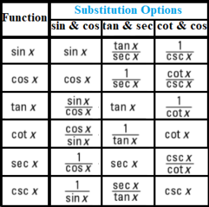
The following table shows how to express one of the common six trig functions as a pair of other trig functions. These may also come in handy:
Trig Substitution: References
Banner, A. (2007). The Calculus Lifesaver: All the Tools You Need to Excel at Calculus (Princeton Lifesaver Study Guides) Illustrated Edition. Princeton University Press.
Jones, J. (2010). Skills Needed for Success in Calculus 1.
Kouba, D. (2017). Finding Integrals Using the Method of Trigonometric Substitution. Retrieved November 9, 2020 from: https://www.math.ucdavis.edu/~kouba/CalcTwoDIRECTORY/trigsubdirectory/TrigSub.html
Related Articles
Change of Variable.
Contour Integral: Simple Definition, Examples
Other References
Iterated Integrals
Contents:
What is an Iterative Process?
Iterated Integral
What is an Iterative Process?
An iterative process is a process which is run over and over again repeatedly, to ultimately reach or approach a desired result. Each cycle, or repetition, is called an iteration. An iterative process may include a finite (fixed) number of iterations with a definite stopping point, or it may go on infinitely.
Iterative Process Examples
As a very simple example, counting by twos is an iterative process, because you’re adding 2 each time, over and over again.
 The Koch snowflake is a more complicated example of an iterative process. The first iteration is an equilateral triangle; each successive iteration is formed by adding smaller equilateral triangles to the first.
A recursive formula is a sequence or quantity that is described by a iterative process.
One recursive formula is the one which describes the Fibonacci sequence. The Fibonacci sequence can be defined as:
- F0 = 0
- F1 = 1
- Fn = Fn-1 + Fn-2
To find the value of a given Fibonacci number, you can run an iterative process, starting from F0 and F1 and finding the next number by repeatedly using the formula Fn = Fn-1 + Fn-2.
Using this formula, F2 is 0 + 1 = 1. To find F4, though, you would need to run several iterations of the formula—first find F2 = 1 and F3 = F2 + F1 = 1 + 1 = 2. For any Fibonacci number n >2, you would have to run n – 1 calculations to find out its value using only the definition above.
Calculating compound interest is another example of iterative processes. If interest is compounded yearly, we find the total interest accumulated in ten years by multiplying, year by year, the interest + 100% by the previous years balance.
Iterated Integrals
An iterated integral has the general form (Rogawski, 2007):
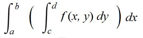
The expression is made up of an “inner integral” and one or more outer integrals. An iterated integral with two integrals is called a double integral; A triple integral is a three integral expression.
Solving the Iterated Integral
An iterated integral is worked much in the same way that inner functions and outer functions are worked in the chain rule for derivatives: you start by evaluating the inner function (or in this case, the inner integral), then work your way out. In other words, you’re performing iterative integration. In the generic example given above, you would integrate with respect to y first (using c, d as the bounds of integration), then work the new integral with respect to x (using a, b as the bounds of integration).
For an example, see: Solving a Double Integral or Solving a Triple Integral.
One of the surprising benefits of iterated integrals is that you can change the order of integration if, for example, the inner integral is impossible to evaluate. While “regular” integration is like slicing a loaf of bread along its length, changing the order of integration allows you to slice across its width instead.
Fubini’s Theorem
Theorems which relate multiple integrals (integrated over subsets of ℝ) to iterated integrals are normally called Fubini Theorems (Swarz, 2001). In simple terms, Fubini’s theorem states:
“…when we have a ‘nice’ function, that the n-dimensional multiple integral of this function is the same as the n-fold iterated integral” (Tollas, 2007).
References
Iteration in Matlab. Retrieved from https://www.mathworks.com/content/dam/mathworks/mathworks-dot-com/moler/exm/chapters/iteration.pdf on January 8, 2018.
Rogawski, J. Multivariable Calculus. W. H. Freeman. 2007.
Rudin, W., Real and complex analysis, 1970. McGraw-Hill Education.
Swarz, C. Introduction to Gauge Integrals. World Scientific. 2001.
Section 12.2/12.3: Iterated Integrals Double Integrals over General Regions. Retrieved July 3, 2020 from: https://www.radford.edu/npsigmon/courses/calculus4/mword/Section12.2-12.3notes.pdf
Tollas, L. (2007). Iterated Integrals. Article posted on Reed College website. Retrieved July 3, 2020 from: https://blogs.reed.edu/projectproject/2017/07/14/iterated-integrals/