Logistic growth is used to measure changes in a population, much in the same way as exponential functions. The model has a characteristic “s” shape, but can best be understood by a comparison to the more familiar exponential growth model.
The word “logistic” doesn’t have any actual meaning—it’s just a commonly accepted name given to this type of growth [1].
Exponential vs. Logistic Growth
Unlike exponential growth where the growth rate is constant and the population grows “exponentially”, in logistic growth a population’s growth rate (not the population itself) decreases as the population size approaches a maximum level. The maximum level is determined by the environment’s finite supply of resources (i.e. the amount of food). The resource limit (i.e. the maximum amount of food available) is known as the carrying capacity (K).
There are some important differences between exponential growth and logistic growth. The graph labeled logistic growth features an s-shaped line reflecting the leveling-off of the growth rate:
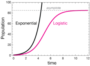
At first, the logistic portion of the graph (in red) growths roughly exponentially. When the population size reaches K/2, the growth rate declines, eventually reaching a horizontal asymptote at carrying capacity K (the breaking agent) [2].
Differential Equations
Like other differential equations, logistic growth has an unknown function and one or more of that function’s derivatives. The standard differential equation is:
![]()
Where:
- K is the carrying capacity,
- Po is the initial density of the population,
- r is the growth rate of the population.
From the above equation we can deduce whether solutions increase or decrease. For example, if the population (P) falls between 0 and K, then the right side of the equation will be positive. This means that dP/dt > 0 so the population increases. In the alternative, if the population (P) exceeds the carrying capacity (P>K), then 1 – P/K will be negative. This tells us that dP/dt < 0 and therefore the population decreases.
Real World Applications for the Logistic Growth Model
There are many real world applications for this type of growth. In addition to examining large scale populations like the human race, we can also analyze animal and even microorganism populations. Logistic Growth is also used commercially to analyze the life-spans of products.
History
P.F. Verhulst was a Belgian mathematician that studied the logistic growth model in the 19th century (and is that namesake behind the second name for the formula, the Verhulst Model). He used the model to predict what the U.S. population would be in 1940. Despite a 100-year gap, his prediction was off by less than 1%.
References
[1] Logistic Growth Model. Retrieved July 14, 2021 from: https://services.math.duke.edu/education/ccp/materials/diffeq/logistic/logi1.html
[2] Lecture notes for ZOO 4400/5400 Population Ecology.
Retrieved July 14, 2021 from: http://www.uwyo.edu/dbmcd/popecol/janlects/lect05.html