Lagrange Interpolating Polynomial: Definition
A Lagrange Interpolating Polynomial is a Continuous Polynomial of N – 1 degree that passes through a given set of N data points. By performing Data Interpolation, you find an ordered combination of N Lagrange Polynomials and multiply them with each y-coordinate to end up with the Lagrange Interpolating Polynomial unique to the N data points. This unique polynomial exactly fits the given set of data points and their constraints. The constraints, for example, can include the rate of change values for each x-coordinate in the data set.
*For simplicity’s sake, we shall only consider the exact set of data points when calculating a Lagrange Interpolating Polynomial.
For a given set {(x1, y1),(x2, y2),…,(xN, yN)}, a Lagrange Interpolating Polynomial is represented as:
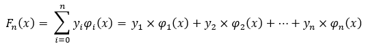
Where the yi‘s are the y-coordinates from the given data set (in respect to their paired x-coordinate) and where each φi (x) are individual Lagrange Polynomials formed by using the x-coordinates from the given N data points. The Lagrange Polynomial equation is:
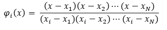
Note that the numerator contains the multiplication of all factors except the factor (x – xi), to which the Lagrange Polynomial is based on, and the denominator contains the multiplication of differences between the xi) and all other x-coordinate values except x)i) itself. These exclusions prevent the fraction from equaling 0 (i.e. “x” being subtracted by the first x-coordinate) and Does Not Exist (i.e. 1 divided by the quantity of the first x-coordinated subtracting itself).
Being one of many Calculus tools used to model discrete data points, the data fitting technique of interpolation guarantees the finding of one unique solution that fits all the given data points exactly. Although the Lagrange Interpolating Polynomial models the data points exactly, all other points that make this polynomial continuous are approximated and thus contain an overall approximation error. The more data points that are introduced to the mathematician, the lower the approximation error value becomes for all points in between the given data set.
Modeling Example
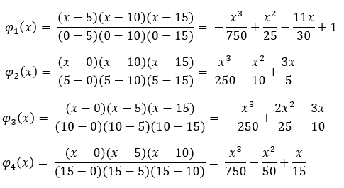
For a data set of N = 4 data points, let the coordinates (0, 15), (5, -5), (10, 30), and (15, 5) represent the set to model. First, the Lagrange Polynomials are calculated for each coordinate we are given:
For each Lagrange Polynomial, their appropriate yi value is multiplied to get the following summation:
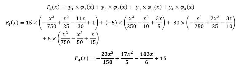
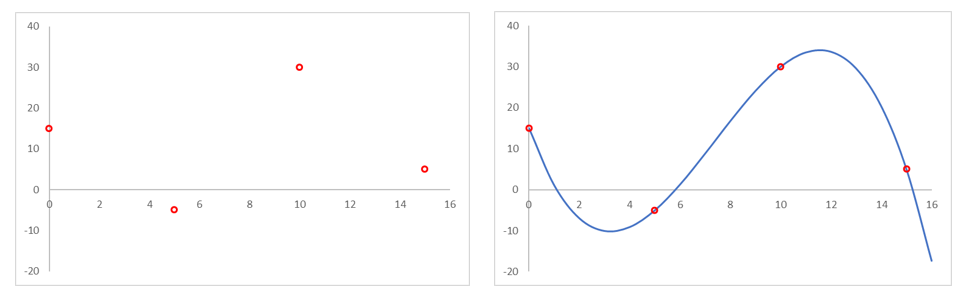
The calculated F4 (x) function does exactly fit the given data set while approximating all points in-between the data set’s coordinates. Understand that F4 (x) only works for the given 4 coordinates and if a 5th data point was introduced, then all the Lagrange Polynomials need to be recalculated.
Data Point Computation Example
If given one x-coordinate to test for a given set of data points, instead of needing to find the specific Lagrange Interpolating Polynomial, the summation of Fn(x) can be calculated in one go.
Using the data set described in the above example, let’s find what F4 (7) equals.
Finding F4 (7) can be written as:
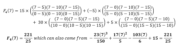
The calculated value for x = 7 is treated as an approximated value within the coordinates (0,15), (5,-5), (10,30), and (15,5). The approximation idea exists only if an original equation (that generated the 4 exact coordinates) was present to compare with. Since the 4 coordinates weren’t based off from an actual polynomial, we can take the coordinate (7, 221/25) as a meaningful data point.
Interpolation Error
The procedure in finding a Lagrange Interpolating Polynomial comes into question when the number of data points within a given set gets too large. Polynomial interpolation starts to lose its small approximation capability since high-degree interpolation can create oscillatory behaviors. Compared to a smooth function, where the number of rises and falls is small, an oscillatory approximation is unreliable in retrieving steady measurement values.
Runge’s Example can best present this for the function f(x) = 1/((1 + x2)) within the domain [-5, 5]. Let 10 equally spaced data points be generated from f(x) to obtain the Lagrange Interpolating Polynomial function:

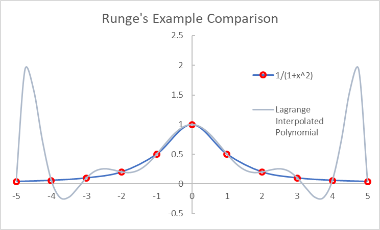
Where each of the 10 coordinates (in red) hit the exact values for both f(x) = 1 / ((1 + x2)) and f10 (x) but differ everywhere else within the domain [-5, 5]. It can be imagined that outside the domain bounds of [-5,5], the Lagrange Interpolating Polynomial’s oscillatory behavior can be equated to that of noise and thus be discarded. Runge’s example sets the scenario for the difficulty in expecting a high-degree polynomial interpolation to represent a large data set for further measurement taking. The creation of Lagrange Interpolating Polynomials is best suited within the domain of a given data set and for data sets of three to seven coordinates.
References
Corless, Robert M., and Leili Rafiee Sevyeri. “The Runge Example for Interpolation and Wilkinsons Examples for Rootfinding.” SIAM Review, vol. 62, no. 1, 2020, pp. 231–243., doi:10.1137/18m1181985.
Deford, D.. Lagrange Interpolation. Retrieved from https://people.csail.mit.edu/ddeford/Lagrange_Interpolation.pdf
Hildebrand, F. B.. “Lagrangian Methods.” Introduction to Numerical Analysis: Second Edition. United States, Dover Publications, 1974. Retrieved from https://archive.org/details/IntroductionToNumericalAnalysis/page/n7/mode/2up