Calculus Definitions > Different Types of Calculus:
- Traditional (Infinitesimal) Calculus
- Non-Newtonian Calculus
- Stochastic Calculus
- Propositional, Ricci, Finite, Lambda & Umbral
Traditional (Infinitesimal) Calculus
The traditional calculus you come across in AP- or single-variable Calculus is also known as infinitesimal calculus. “Calculus” originally meant accounting or reckoning, originating with the Latin name for a small counting pebble.
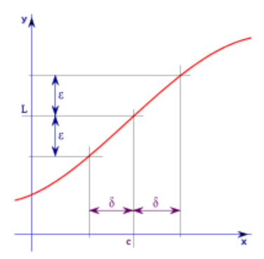
Infinitesimal calculus is a formal system of calculation, involving two major branches: derivatives (the slope of a tangent line at a point) and integrals (a way to find the area under the curve). However, there are dozens of different types of calculus including vector calculus for three-dimensional (or higher) curves, surfaces and solid bodies and exterior calculus , a high-dimensional calculus which is particularly well suited for working in complex analysis.
Some of the other different types of calculus make small changes to the way the calculations are performed, like switching small additive changes to small multiplicative changes. Other types of “calculus” are far removed from the traditional calculus of Newton and Leibniz, spreading over to fields like mathematical logic.
To muddy the waters a little, there is another branch of calculus called nonstandard calculus. Despite the name, it doesn’t mean “non-traditional calculus”; It refers to a small branch of calculus that applies quite technical (and difficult to understand for many) nonstandard analysis tools to infinitesimal calculus.
Real Analysis

Essentially, you go from the “what” in calculus is true to “why” it’s true (Lebl, 2020).
What is Taught in Real Analysis?
A typical real analysis course includes:
- Construction and properties of real numbers. For example, cardinality, algebraic and order structures of real and rational number systems.
- Introduction to logical structures and construction of proofs.
- Core calculus topics: limits, continuity, differentiation and the Riemann integrals—with a heavy emphasis on proofs.
- Sequences and series: introduced in calculus, these are heavily emphasized in real analysis.
- Introduction to differential equations.
Real analysis heavily emphasizes proofs. In fact, you can barely take a step in the course without axioms and postulates: every formula encountered in the class has to be proved. Instead of using formulas for derivatives and integration, you’ll be proving that they work.
What Are Some Uses for Real Analysis?
Real analysis underpins many other branches of mathematics including probability theory and analytic number theory. However, it isn’t just a scholarly exercise in pedantry. Real world uses include:
- Describing physical systems with ordinary differential equations,
- Formulating optimal structures (minimums, maximums, and equilibriums),
References
Lebl, J. (2020). Basic Analysis I. Retrieved September 20, 2020 from: https://www.jirka.org/ra/realanal.pdf
Bloch, E. (2011). The Real Numbers and RA. Springer.
Schramm, M. (2012). Introduction to RA. Dover Publications.
MCMullen, C. Course Notes. Retrieved September 20, 2020 from: http://people.math.harvard.edu/~ctm/papers/home/text/class/harvard/114/course/course.pdf
Trench, W. (2013). Introduction to RA (TRENCH_REAL_ANALYSIS).
Different Types of Calculus #1: Non-Newtonian Calculus
Unlike traditional calculus, which is linear with additive operators, Non-Newtonian calculus is non-linear and lacks additive operators. For example, exponential calculus (also called geometric calculus) has multiplicative operators. These operators can only be applied to positive functions, so only positive functions are valid in this particular calculus.
Grossman & Katz [1] outlined several branches, including multiplicative calculus, which uses multiplicative (instead of additive) operators. One sub branch is bigeometric calculus, where ratios measure changes in arguments and values and products are used for accumulations. Other lesser known branches of non-Newtonian calculus include: Anageometric, Biquadratic, and Harmonic calculus.
Different Types of Calculus #2: Stochastic Calculus
Stochastic calculus deals with stochastic (random) processes or equations that involve statistical noise. It’s a blend of probability and calculus which allows us to apply the principles of calculus to events with random elements. Problems in the field are defined by algebraic, integral, or differential equations with random coefficients or inputs [1].
Key Elements of Stochastic Calculus
A key part of stochastic calculus is Brownian motion, named after Robert Brown’s observation of the random walk pollen particles take when suspended in water. Brownian motion is actually a blend of several random and non-random elements: it is part Gaussian, part martingale and part Markov process (a random process where the future is independent of the past). The paths of Brownian motion are irregular and nowhere differentiable [2], making them impossible to study in “regular” calculus. Later on, Norbert Weiner made mathematical sense of the apparently random motion; This led to the development of a limiting stochastic process called the Weiner process[3], which is now used to model Brownian motion.
Another element of stochastic calculus is the Ito integral, defined as:
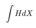
Where:
- H = a locally bounded predictable process,
- X = a semimartingale.
This new type of integral was developed because Brownian motion is not of bounded variation— a requirement of the usual Riemann integral.
The stochastic differential equation (SDE) also plays a key role. It is defined as:
dXt = b(Xt)dt + σ(Xt) dBt
Where:
- Bt = one-dimensional Brownian motion.
One way to think of this is as the differential equation dXt/dt = b(Xt) perturbed by noise. The most well-known use of the stochastic differential equation is in modeling stock prices [4].
Stochastic Calculus: References
[1] Grigoriu, M. (2002). Stochastic Calculus: Applications in Science and Engineering. Birkhauser.
[2] Stochastic Calculus. Retrieved April 18, 2021 from: https://www.math.purdue.edu/~stindel/teaching/stoch-calc/stoch-calc.html
[3] Van Handel, R. (2007). Stochastic Calculus, Filtering, and
Stochastic Control. Retrieved April 18, 2021 from: https://web.math.princeton.edu/~rvan/acm217/ACM217.pdf
[4] Cohen, S. & Elliot, R. (2015). Stochastic Calculus and Applications. Birkhauser.
Propositional, Ricci, Finite, Lambda & Umbral
Some branches of calculus are used for very narrow purposes. For example:
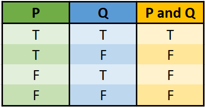
- Propositional calculus (also called sentential calculus) is a types of symbolic logic—a way to analyze truth relationships via statements like and, or, not and if.

A truth table used in propositional calculus.
This calculi is the foundational of most logical-mathematical theories; Predicate Calculus is a more complex version, allowing functions, relations, and quantifiers [2]. - Ricci calculus, also called the calculus of congruences of curves [1], is the study of tensors and tensor fields.
- Finite calculus (also called calculus of finite differences) is calculus for discrete values. It useful for many areas like marginal economic analysis, growth and decay, and modeling human behavior.
- Lambda calculus is made up a transformation rule and a function definition scheme. It is used extensively in higher-order logic and computer programming, where it forms the underpinnings of many computer programs (like LISP).
- Umbral calculus (also called Blissard Calculus or Symbolic Calculus) is a modern way to do algebra on polynomials. Generally speaking, it’s a way to discover and prove combinatorial identities, but it can also be viewed as a theory of polynomials that count combinatorial objects [3].
References
[1] Grossman M., Katz R., (1972), Non-Newtonian Calculus, Lee Press, Piegon Cove, Massachusetts.
[2] Goldmakher, L. (2020). Propositional and Predicate Calculus.
[3] Ray, N. Universal Constructions in Umbral Calculus. Retrieved May 4, 2021 from: http://www.ma.man.ac.uk/~nige/ucuc.pdfH.