Probability and Statistics > Regression analysis
Regression analysis is a way to find trends in data. For example, you might guess that there’s a connection between how much you eat and how much you weigh; regression analysis can help you quantify that.
Regression analysis will provide you with an equation for a graph so that you can make predictions about your data. For example, if you’ve been putting on weight over the last few years, it can predict how much you’ll weigh in ten years time if you continue to put on weight at the same rate. It will also give you a slew of statistics (including a p-value and a correlation coefficient) to tell you how accurate your model is. Most elementary stats courses cover very basic techniques, like making scatter plots and performing linear regression. However, you may come across more advanced techniques like multiple regression.
Contents:
- Introduction to Regression Analysis
- Multiple Regression Analysis
- Overfitting and how to avoid it
- Related articles
Technology:
Regression Analysis: An Introduction
In statistics, it’s hard to stare at a set of random numbers in a table and try to make any sense of it. For example, global warming may be reducing average snowfall in your town and you are asked to predict how much snow you think will fall this year. Looking at the following table you might guess somewhere around 10-20 inches. That’s a good guess, but you could make a better guess, by using regression.
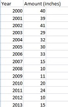
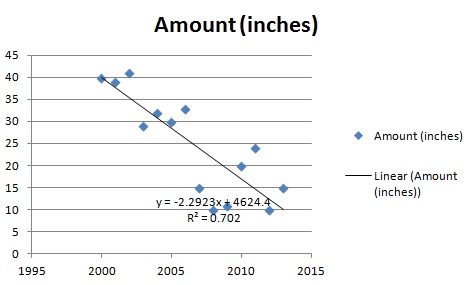
Essentially, regression is the “best guess” at using a set of data to make some kind of prediction. It’s fitting a set of points to a graph. There’s a whole host of tools that can run regression for you, including Excel, which I used here to help make sense of that snowfall data:
Just by looking at the regression line running down through the data, you can fine tune your best guess a bit. You can see that the original guess (20 inches or so) was way off. For 2015, it looks like the line will be somewhere between 5 and 10 inches! That might be “good enough”, but regression also gives you a useful equation, which for this chart is:
y = -2.2923x + 4624.4.
What that means is you can plug in an x value (the year) and get a pretty good estimate of snowfall for any year. For example, 2005:
y = -2.2923(2005) + 4624.4 = 28.3385 inches, which is pretty close to the actual figure of 30 inches for that year.
Best of all, you can use the equation to make predictions. For example, how much snow will fall in 2017?
y = 2.2923(2017) + 4624.4 = 0.8 inches.
Regression also gives you an R squared value, which for this graph is 0.702. This number tells you how good your model is. The values range from 0 to 1, with 0 being a terrible model and 1 being a perfect model. As you can probably see, 0.7 is a fairly decent model so you can be fairly confident in your weather prediction!
Multiple Regression Analysis
Multiple regression analysis is used to see if there is a statistically significant relationship between sets of variables. It’s used to find trends in those sets of data.
Multiple regression analysis is almost the same as simple linear regression. The only difference between simple linear regression and multiple regression is in the number of predictors (“x” variables) used in the regression.
- Simple regression analysis uses a single x variable for each dependent “y” variable. For example: (x1, Y1).
- Multiple regression uses multiple “x” variables for each independent variable: (x1)1, (x2)1, (x3)1, Y1).
In one-variable linear regression, you would input one dependent variable (i.e. “sales”) against an independent variable (i.e. “profit”). But you might be interested in how different types of sales effect the regression. You could set your X1 as one type of sales, your X2 as another type of sales and so on.
When to Use Multiple Regression Analysis.
Ordinary linear regression usually isn’t enough to take into account all of the real-life factors that have an effect on an outcome. For example, the following graph plots a single variable (number of doctors) against another variable (life-expectancy of women).
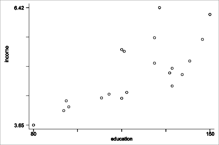
From this graph it might appear there is a relationship between life-expectancy of women and the number of doctors in the population. In fact, that’s probably true and you could say it’s a simple fix: put more doctors into the population to increase life expectancy. But the reality is you would have to look at other factors like the possibility that doctors in rural areas might have less education or experience. Or perhaps they have a lack of access to medical facilities like trauma centers.
The addition of those extra factors would cause you to add additional dependent variables to your regression analysis and create a multiple regression analysis model.
Multiple Regression Analysis Output.
Regression analysis is always performed in software, like Excel or SPSS. The output differs according to how many variables you have but it’s essentially the same type of output you would find in a simple linear regression. There’s just more of it:
- Simple regression: Y = b0 + b1 x.
- Multiple regression: Y = b0 + b1 x1 + b0 + b1 x2…b0…b1 xn.
The output would include a summary, similar to a summary for simple linear regression, that includes:
- R (the multiple correlation coefficient),
- R squared (the coefficient of determination),
- adjusted R-squared,
- The standard error of the estimate.
These statistics help you figure out how well a regression model fits the data. The ANOVA table in the output would give you the p-value and f-statistic.
Minimum Sample size
“The answer to the sample size question appears to depend in part on the objectives
of the researcher, the research questions that are being addressed, and the type of
model being utilized. Although there are several research articles and textbooks giving
recommendations for minimum sample sizes for multiple regression, few agree
on how large is large enough and not many address the prediction side of MLR.” ~ Gregory T. Knofczynski
If you’re concerned with finding accurate values for squared multiple correlation coefficient, minimizing the
shrinkage of the squared multiple correlation coefficient or have another specific goal, Gregory Knofczynski’s paper is a worthwhile read and comes with lots of references for further study. That said, many people just want to run MLS to get a general idea of trends and they don’t need very specific estimates. If that’s the case, you can use a rule of thumb. It’s widely stated in the literature that you should have more than 100 items in your sample. While this is sometimes adequate, you’ll be on the safer side if you have at least 200 observations or better yet—more than 400.
Overfitting in Regression
Overfitting is where your model is too complex for your data — it happens when your sample size is too small. If you put enough predictor variables in your regression model, you will nearly always get a model that looks significant.
While an overfitted model may fit the idiosyncrasies of your data extremely well, it won’t fit additional test samples or the overall population. The model’s
p-values, R-Squared and regression coefficients can all be misleading. Basically, you’re asking too much from a small set of data.
How to Avoid Overfitting
In linear modeling (including multiple regression), you should have at least 10-15 observations for each term you are trying to estimate. Any less than that, and you run the risk of overfitting your model.
“Terms” include:
- Interaction Effects,
- Polynomial expressions (for modeling curved lines),
- Predictor variables.
While this rule of thumb is generally accepted, Green (1991) takes this a step further and suggests that the minimum sample size for any regression should be 50, with an additional 8 observations per term. For example, if you have one interacting variable and three predictor variables, you’ll need around 45-60 items in your sample to avoid overfitting, or 50 + 3(8) = 74 items according to Green.
Exceptions
There are exceptions to the “10-15” rule of thumb. They include:
- When there is multicollinearity in your data, or if the effect size is small. If that’s the case, you’ll need to include more terms (although there is, unfortunately, no rule of thumb for how many terms to add!).
- You may be able to get away with as few as 10 observations per predictor if you are using logistic regression or survival models, as long as you don’t have extreme event probabilities, small effect sizes, or predictor variables with truncated ranges. (Peduzzi et al.)
How to Detect and Avoid Overfitting
The easiest way to avoid overfitting is to increase your sample size by collecting more data. If you can’t do that, the second option is to reduce the number of predictors in your model — either by combining or eliminating them. Factor Analysis is one method you can use to identify related predictors that might be candidates for combining.
1. Cross-Validation
Use cross validation to detect overfitting: this partitions your data, generalizes your model, and chooses the model which works best. One form of cross-validation is predicted R-squared. Most good statistical software will include this statistic, which is calculated by:
- Removing one observation at a time from your data,
- Estimating the regression equation for each iteration,
- Using the regression equation to predict the removed observation.
Cross validation isn’t a magic cure for small data sets though, and sometimes a clear model isn’t identified even with an adequate sample size.
2. Shrinkage & Resampling
Shrinkage and resampling techniques (like this R-module) can help you to find out how well your model might fit a new sample.
3. Automated Methods
Automated stepwise regression shouldn’t be used as an overfitting solution for small data sets. According to Babyak (2004),
“The problems with automated selection conducted in this very typical manner are so
numerous that it would be hard to catalogue all of them [in a journal article].”
Babyak also recommends avoiding univariate pretesting or screening (a “variation of automated selection in disguise”), dichotomizing continuous variables — which can dramatically increase Type I errors, or multiple testing of confounding variables (although this may be ok if used judiciously).
References
Books:
Gonick, L. (1993). The Cartoon Guide to Statistics. HarperPerennial.
Lindstrom, D. (2010). Schaum’s Easy Outline of Statistics, Second Edition (Schaum’s Easy Outlines) 2nd Edition. McGraw-Hill Education
Journal articles:
- Babyak, M.A.,(2004). “What you see may not be what you get: a brief, nontechnical introduction to overfitting in regression-type models.” Psychosomatic Medicine. 2004 May-Jun;66(3):411-21.
- Green S.B., (1991) “How many subjects does it take to do a regression analysis?” Multivariate Behavior Research 26:499–510.
- Peduzzi P.N., et. al (1995). “The importance of events per independent variable in multivariable analysis, II: accuracy and precision of regression estimates.” Journal of Clinical Epidemiology 48:1503–10.
- Peduzzi P.N., et. al (1996). “A simulation study of the number of events per variable in logistic regression analysis.” Journal of Clinical Epidemiology 49:1373–9.
Check out our YouTube channel for hundreds of videos on elementary statistics, including regression analysis using a variety of tools like Excel and the TI-83.
More articles
- Additive Model & Multiplicative Model
- How to Construct a Scatter Plot.
- How to Calculate Pearson’s Correlation Coefficients.
- How to Compute a Linear Regression Test Value.
- Chow Test for Split Data Sets
- Forward Selection
- What is Kriging?
- How to Find a Linear Regression Equation.
- How to Find a Regression Slope Intercept.
- How to Find a Linear Regression Slope.
- Sinusoidal Regression: Definition, Desmos Example, TI-83
- How to Find the Standard Error of Regression Slope.
- Mallows’ Cp
- Validity Coefficient: What it is and how to find it.
- Quadratic Regression.
- Quantile Regression In Analysis
- Quartic Regression
- Stepwise Regression
- Unstandardized Coefficient
- Next:: Weak Instruments
Fun fact: Did you know regression isn’t just for creating trendlines. It’s also a great hack for finding the nth term of a quadratic sequence.
Definitions
- ANCOVA.
- Assumptions and Conditions for Regression.
- Betas / Standardized Coefficients.
- What is a Beta Weight?
- Bivariate correlation and regression.
- Bilinear Regression
- The Breusch-Pagan-Godfrey Test
- Cook’s Distance.
- What is a Covariate?
- Cox Regression.
- Detrend Data.
- Exogeneity.
- Gauss-Newton Algorithm.
- What is the General Linear Model?
- What is the Generalized Linear Model?
- What is the Hausman Test?
- What is Homoscedasticity?
- Influential Data.
- What is an Instrumental Variable?
- Lack of Fit
- Lasso Regression.
- Levenberg–Marquardt Algorithm
- What is the Line of best fit?
- What is Logistic Regression?
- What is the Mahalanobis distance?
- Model Misspecification.
- Multinomial Logistic Regression.
- What is Nonlinear Regression?
- Ordered Logit / Ordered Logistic Regression
- What is Ordinary Least Squares Regression?
- Overfitting.
- Parsimonious Models.
- What is Pearson’s Correlation Coefficient?
- Poisson Regression.
- Probit Model.
- What is a Prediction Interval?
- What is Regularization?
- Regularized Least Squares.
- Regularized Regression
- What are Relative Weights?
- What are Residual Plots?
- Reverse Causality.
- Ridge Regression
- Root Mean Square Error.
- Semiparametric models
- Simultaneity Bias.
- Simultaneous Equations Model.
- What is Spurious Correlation?
- Structural Equations Model
- What are Tolerance Intervals?
- Trend Analysis
- Tuning Parameter
- What is Weighted Least Squares Regression?
- Y Hat explained.
Regression in Minitab
Regression is fitting data to a line (Minitab can also perform other types of regression, like quadratic regression). When you find regression in Minitab, you’ll get a scatter plot of your data along with the line of best fit, plus Minitab will provide you with:
- Standard Error (how much the data points deviate from the mean).
- R squared: a value between 0 and 1 which tells you how well your data points fit the model.
- Adjusted R2 (adjusts R2 to account for data points that do not fit the model).
Regression in Minitab takes just a couple of clicks from the toolbar and is accessed through the Stat menu.
Example question: Find regression in Minitab for the following set of data points that compare calories consumed per day to weight:
Calories consumed daily (Weight in lb): 2800 (140), 2810 (143), 2805 (144), 2705 (145), 3000 (155), 2500 (130), 2400 (121), 2100 (100), 2000 (99), 2350 (120), 2400 (121), 3000 (155).
Step 1: Type your data into two columns in Minitab.
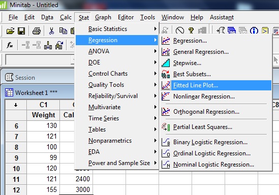
Step 2: Click “Stat,” then click “Regression” and then click “Fitted Line Plot.”
Step 3: Click a variable name for the dependent value in the left-hand window. For this sample question, we want to know if calories consumed affects weight, so calories is the independent variable (Y) and weight is the dependent variable (X). Click “Calories” and then click “Select.”
Step 4: Repeat Step 3 for the dependent X variable, weight.
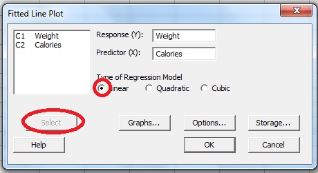
Step 5: Click “OK.” Minitab will create a regression line graph in a separate window.
Step 4: Read the results. As well as creating a regression graph, Minitab will give you values for S, R-sq and R-sq(adj) in the top right corner of the fitted line plot window.
s = standard error.
R-Sq = Coefficient of Determination
R-Sq(adj) = Adjusted Coefficient of Determination (Adjusted R Squared).
That’s it!