The terms sequence and series sound very similar, but they are quite different. Basically:
- A sequence is a set of ordered numbers, like 1, 2, 3, …,
- A series is the sum of a set of numbers, like 1 + 2 + 3….
Sequence and Series: Contents:
- Sequence Definition
- Sequence Rules
- Types of Sequences:
- Arithmetic Progression
- Arithmetic Sequence
- Bounded Sequence
- Cauchy Sequence
- Complementary Sequence
- Complete Sequence
- Constant Sequence, Eventually Constant
- Ducci Sequence
- Exponential Sequence
- Fibonacci Sequence
- Finite Geometric Sequence
- Finite Sequence
- Generating Sequence / Function
- Increasing Sequence
- Infinite Sequence
- Infinite Geometric Sequence
- Integer Sequence
- Monotonic Sequence / Series
- n-tuple
- Numeric Sequence
- Periodic Sequence, Purely / Ultimately
- Polynomial Sequence
- Quadratic Sequence
- Random Sequence
- Recamán Sequence
- Recursive Definition of a Sequence
- Sequence of Partial Sums
- Stationary Sequence: Weakly/Strongly
- Universal Sequence
- What is a Series?
- Types of Series:
- Alternating Series
- Arctangent Series Expansion
- Asymptotic Series / Poincaré Expansion
- Binomial Series
- Continuous Series & Discrete Series
- Dirichlet Series
- Divergent Series
- Finite Series
- Fractional Power Series: Definition, Examples
- Fourier Series
- Geometric Series
- Harmonic Series, Alternating Harmonic Series
- Infinite Series
- Laurent Series
- Monotonic Sequence / Series
- Mercator Series
- Oscillating Series
- P-Series
- Positive Series
- Power Series
- Stirling Series
- Telescoping Series
- Trigonometric Series
Related articles:
- Asymptotic Error (Rate of Convergence)
- Cauchy Convergence
- Find the Limit of a Sequence
- Monotone Convergence Theorem: Examples, Proof
- Series Expansions.
- Sequence of Functions
- Subsequential Limit
- Sum of a Series: How to Find
What is a Sequence?

A sequence is a collection of elements (usually numbers) with two major differences from plain old “sets”:
- The elements (or terms) are in order.
- The values of the terms can repeat.
The number of elements is called the length of the sequence. The length is potentially infinite, meaning it goes on without end. If the collection of numbers ends then it is called a finite sequence.
Sequence Rules and Arithmetic Sequences
Sequences generally have a rule. The rule is applied to find the value of unknown terms. For example, the sequence {3, 6, 9, 12…} begins at 3 and increases by 3 for every subsequent value. This is an example of an arithmetic sequence with a common difference of 3.
The above rule is helpful in defining values in the immediate vicinity of the preceding terms. A limitation of the rule, however, is that it does not tell us the value of an unknown term. In the example above, we don’t know what the 100th term will be. In other words, we need a rule that can quickly determine the value for any unknown term.
Formula and Example for Nth Term
The formula for the nth term of the arithmetic sequence (also called the general term) is:
An = a + (n -1)d
Where:
- an is the nth term of the sequence,
- a is the first term,
- d is the common difference.
The nth term is the unknown term that you are trying to calculate. Using the formula above you can quickly calculate any nth term.
Example question: Find the 100th term for {3, 6, 9, 12…}:
Step 1: Determine the values for an, d and n.
- an (the nth term that you are trying to find) = 100,
- a is the first term: 3,
- d is the common difference (3),
Step 2: Place each value from Step 1 into the formula:
- a100 = 3 + (100 – 1) 3
- = 3 + (99) 3
- = 3 + 297
a100 = 300
The 100th term is 300.
Arithmetic Progression
An arithmetic progression (or arithmetic sequence) is a list of numbers, where every term increases by the same amount—called a common difference. In other words, to go from one term to the next, you just add a number. For example, starting with 1:
- {1, 2, 3} … add 1 each time,
- {1, 7, 14} … add 7 each time.
You don’t have to start with 1 though; You can start with any number. What’s important is that you add the same constant each time.
Finding Common Difference in Arithmetic Progression
The common difference is how much is added to each term in the sequence. For example, the sequence {2, 4, 6, 8} increases by 2—the common difference. Another example: {1, 25, 49} has a common difference of 24. In notation, the common difference is often written as d. For example:
a, a + d, a + 2d, a + 3d, a + 4d.
Which can also be written as a + (n · d), where n starts at zero.
For example, if a = 1 and d = 2:
1, 1 + 2, 1 + 2(2), 1 + 3(2), 1 + 4(2) = 1, 2, 5, 7, 9.
Example question: What is the common difference for the arithmetic progression {5, 8, 11, 14, 17}?
Step 1: Identify the first term. In this list, that’s 5.
Step 2: Subtract the first term from the second: 8 – 5 = 3.
The common difference is 3.
Finite and Infinite Arithmetic Progression
The progression can be a fixed (finite) amount of numbers or an infinite amount. For example, starting with 2 and using a common difference of 3, you get the arithmetic sequence {2, 5, 8, 11…}. The three dots (…) indicate that the sequence goes on an on until infinity. When you have a fixed number of terms, the sequence is called an n-term arithmetic progression. For example, the sequence {2, 5, 8} is a three term arithmetic sequence.
Arithmetic Progression Examples from Number Theory
Arithmetic progression is heavily used in number theory—especially in the analysis of prime numbers. A rather more complex example of an arithmetic progression from number theory:
{a + mk: k >0} ⊆
Where:
- m = fixed integer > 0 &
- a = fixed integer ≥ 0
- Where:
- a + mk = equals a prime number,
- gcd(a, m) = 1.
- Where:
- ⊆ = subset of (or equal to),
- k = a natural number,
- ℕ = set of natural numbers.
The above example is called Dirichlet’s theorem on primes in arithmetic progressions (Lozano-Robledo, 2019). Related to Dirichlet’s theorem are these two important examples of arithmetic progression, which contain all prime numbers except for 2 and 3 (Caldwell, 2020):
- 1, 7, 13, 19, 25, 31, 37, …
- 5, 11, 17, 23, 29, 35, 41, …
Complementary Sequence
A complementary sequence is the inverse of a strictly increasing sequence of non-negative integers (the counting numbers, 1, 2, 3…). “Inverse” refers to the fact it contains numbers not in the original sequence.
More specifically, if a natural-numbered sequence (an) is a strictly increasing sequence of non-negative integers then the complementary sequence is the set of all non-negative integers which are not terms of the sequence [1].
A sequence of positive integers and its complement contain all possible positive integers.
Example of a Complementary Sequence
The complementary sequence of even non-negative integers {2, 4, 6, 8, …} is the odd non-negative integer sequence {1, 3, 5, 7, …}.
This also works in reverse: The complementary sequence of {1, 3, 5, 7, …} is the sequence {2, 4, 6, 8, …}.
Complementary Sequence in Biology
The definition of a complementary sequence in biology is slightly different than the mathematical definition, but the principal is the same. In a way, you can think of them as opposites.
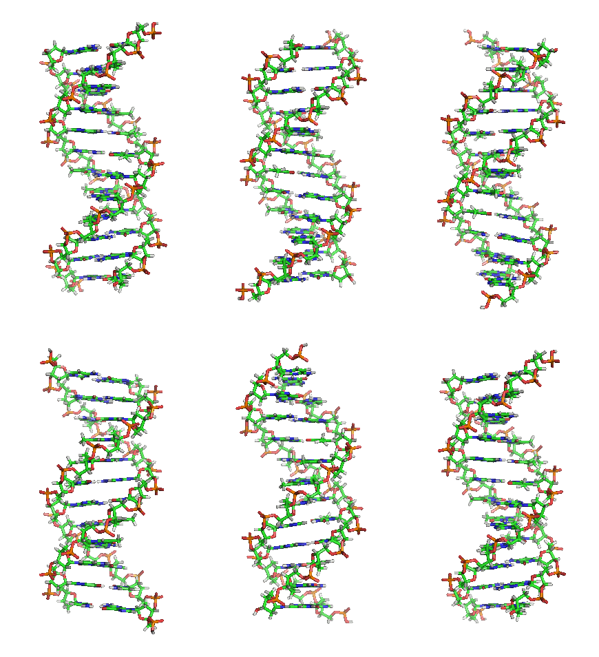
There is a similar complementarity with RNA: Adenine complements Uracil and Guanine complements Cytosine [5].
A pair of Golay complementary sequences is a pair (a, b) of sequences with out-of-phase (i.e. shifts) autocorrelations equal to zero. In other words, Ca(u) + Cb(u) = 0, 0 < u < n [2]. For example, (1 1 -1 1) and (1 1 1 -1) are a Golay complementary pair [3]. These sequences have many applications, including infrared multislit spectrometry and Orthogonal Frequency-Division Multiplexing.
References
[1] Mortich, S. (2010). Remarks on Complementary Sequences. Retrieved April 10, 2021 from: https://www.fq.math.ca/Papers1/48-4/Mortici.pdf
[2] Fieldler, F. & Jedwab, J. (2006). How Do More Golay Sequences Arise? Retrieved April 10, 2021 from: https://www.sfu.ca/~jed/Papers/Fiedler%20Jedwab.%20More%20Golay%20Sequences.%202006.pdf
[3] Kalashnikov, E. (2014). An Introduction to Golay Complementary Sequences. Retrieved April 10 2021 from:https://journals.library.ualberta.ca/eureka/index.php/eureka/article/view/22829
[4] Wellcome Genome Campus Advanced Courses and Scientific Conferences. Grammatical rules for DNA sequence representation. https://www.futurelearn.com/info/courses/bacterial-genomes-bioinformatics/0/steps/47002
[5] Laventa, R. & Cesarini, G. (1981). Base pairing of RNA I with its complementary sequence in the primer precursor inhibits ColE1 replication. Nature 294. 623-626.
Image: Zephyris, CC BY-SA 3.0
Complete Sequence
An increasing sequence of positive integers is a complete sequence if every term can be written as a sum of the first term, using the first term at most once [1].
A couple of variations on this definition:
- Schissel [2] states that a complete sequence if every positive integer is a sum of “one or more distinct terms” in the sequence.
- Erdos & Graham [3] describe a complete sequence as one where “every
sufficiently large” natural number is a sum of distinct terms of the sequence. This particular definition is called a weakly complete sequence [4]. - Linz & Jones [5] define a r-complete sequence, where every sufficiently large positive integer can be represented as the sum of r or more distinct terms from the sequence.
Complete Sequence Examples
A simple example of a complete sequence is {1, 2, 3, 4, …}.
Some complete sequences are more challenging to spot. For example, {1, 2, 3, 4, 8, 12, 16, 20, 24, 28, …} meets the definition because we can represent positive integers in modulo 4 (an arbitrary positive integer, a, can always be written as a = n * q + r).
The prime numbers are a complete sequence (if you add 1).
The Fibonacci sequence {1, 1, 2, 3, 5, 8, …} is an example of a complete sequence. Here [2],
- fl, 1 (1) = 1, f1, 1(2) = 1, and
- f1, 1(n) = f1, 1(n – 1) + f1, 1(n – 2) if n ≥ 3.
Removing a single number still leaves a complete sequence, although removing two numbers does not [6].
Complete Sequence: References
[1] Earl, R. (2017). Towards Higher Mathematics: A Companion. Cambridge University Press.
[2] Schissel , E. (!987). Characterizations of Three Types of Completeness. Retrieved April 7, 2021 from: https://www.fq.math.ca/Scanned/27-5/schissel.pdf
[3] Erdos, P. & Graham, R. (1980). Old and New Problems and Results in Combinatorial Number Theory: Monographie Numero 28 de L’Enseignement Math&matique .
Lf Enseignement Mathematique de 1’Universite de Geneve.
[4] Fox, A. & Knapp, M. (2013). A Note on Weakly Complete Sequences. Journal of Integer Sequences.
[5] Linz, W. & Jones, E. (2016). r-Completeness of Sequences of Positive Integers. Retrieved April 7, 2021 from: https://www.emis.de/journals/INTEGERS/papers/q59/q59.pdf
[6]Honsberger, R. Mathematical Gems III. Washington, DC: Math. Assoc. Amer., 1985.
Ducci Sequence
A Ducci sequence (or N-number game) is a sequence of n-tuples (i.e. a list of integers). Each term in the sequence is formed by finding the absolute difference of neighboring integers [1].
Ducci Sequence Example
Example question: Create a Ducci sequence for the n-tuple (8, 11, 2, 7).
Step 1: Label the n-tuple’s terms a to n:
- a = 8
- b = 11
- c = 2
- d = 7.
Step 2: Subtract pairs of terms (a and b, b and c, c and d …). The last term is paired with the first time, so in this example d will be subtracted from a:
- a – b = 8 – 11 = -3
- b – c = 11 – 2 = 9
- c – d = 2 – 7 = -5
- d – a = 7 – 8 = 1.
Step 3: Place the terms from Step 2 into a new n-tuple, ignoring the negative signs (by taking the absolute value):
(3, 9, 5, 1).
Step 4: Connect the new n-tuples from Step 3 with the Ducci sequence so far. We started with (8, 11, 2, 7), so:
(8, 11, 2, 7) → (3, 9, 5, 1).
Step 5: Repeat Steps 1 to 4 until the sequence wither reaches an n-tuple of all zeros or a periodic (repeating loop):
(8, 11, 2, 7) → (3, 9, 5, 1) → (6, 4, 4, 2) → (2, 0, 2, 4) → (2, 2, 2, 1) → (0, 0, 0, 0).
That’s it!
A Graphical Ducci Sequence
The Ducci sequence can also be calculated using squares or circles, although you should start with a large enough shape (perhaps a whole sheet of paper) so that you don’t run out of room.
Example #2: Create a graph for the Ducci sequence (6, 9, 0, 5)
Step 1: Draw a circle and, starting at the top, write the sequence in a clockwise direction.
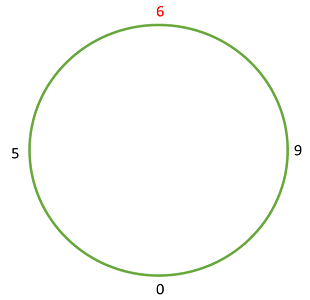
I’ve highlighted the first term of each iteration in red, so that it will be easier to reconstruct the sequence when we’ve finished.
Step 2: Subtract pairs of terms, starting with the red term and moving in a clockwise direction. Write down the absolute value of each difference:
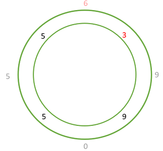
Make sure to highlight the first term, which is 6 – 9 = 3 in this example.
Step 3: Complete the sequence, repeating Step 2 until you get all zeros or have a periodic sequence:
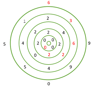
Ducci Sequence: References
[1] 4723 Ducci Sequence. Retrieved May 5, 2021 from: https://icpcarchive.ecs.baylor.edu/external/47/4723.pdf
What is a Generating Sequence?
A generating sequence (also called a generating function) is one way to create a finite sequence.
For example:
- The generating sequence an = cn * rn results in the geometric series if the cns are constant [1].
- The sequence {6, 26, 66} is generated by the formula [x(x2 + 4x + 1)].
The most important reason for finding the generating function for a sequence is that functions have a much larger “toolbox” to work with. For example, you can’t find derivatives and integrals of sequences, but you can apply those procedures to functions.
Not all sequences have generating sequences. For example, it’s not possible explicitly generate an infinite sequence, but you can generate one for a part of it by using a partial sum [2]. For example, the nth partial sum of the generating sequence an is [3]:
![]()
Ordinary Generating Function
The ordinary generating function specifically refers to a formal power series, where the coefficients correspond to a sequence. The general form is:

Which can also be written as:
G(x) = g0 + g1x + g2x2 + g3x3 + ….
The ordinary generating function is a “formal” power series because the x is used as a placeholder instead of a number; In rare circumstances you might put a value in for x, but leaving the placeholder in means that you can ignore the issue of convergence. [4] It is primarily used in computer science and mathematical analysis.
Other Meanings of “Generating Function”
The term “generating function” is loosely defined. Sometimes it’s used as a synonym for the generating sequence described above. To avoid this confusion, the generating function that specifically generates sequences is sometimes called a function for generating sequences .
Alternatively, it could refer to a specific type of computational tool. For example:
- Moment Generating Functions (MGFs) are an alternative way to represent probability distributions; Each distribution has a unique MGF. They are used to find moments like the mean(μ) and variance(σ2).
- Probability Generating Functions are very similar to MGFs and contain the same information. However, the PGF is usually concerned with non-negative, integer-valued random variables.
- A Cumulant Generating Function (CGF) takes the moment of a numerical sequence.
Generating Function: References
[1] Chapter 2: Limits of Sequences.
[2] Basic Calculus Concepts.
[3] Limits of Sequences.
[4] Meyer, A. & Rubinfeld, R. (2005). Generating Functions. Retrieved April 4, 2021 from: https://www.math.cmu.edu/~lohp/docs/math/2011-228/mit-ocw-generating-func.pdf
Increasing Sequence
An increasing sequence increases as you travel along the number line.
In notation:
- a1 ≤ a2 … or
- an ≤ an+1 [1].
In other words, the second term is larger than or equal to the first term, the third term is larger or equal to the second, and so on.
The above definition poses a small problem in that it can define a sequence where the numbers are all equal to each other. When this happens, it’s usually called a constant sequence instead. In order to be a true “increasing sequence”, at least one of the terms in the sequence has to be larger than the one before it. For example:
- Constant sequence: {1, 1, 1, 1, 1}
- Increasing sequence: {1, 1, 1, 1, 2}
Some authors use the term non-decreasing sequence to describe an increasing sequence and strictly increasing to describe increasing sequences. This may be more intuitive, because a constant sequence is certainly non-decreasing. However, all the different terminology can get a little confusing; Make sure you understand exactly what definition your textbook author (or professor) is using.
Monotonically Increasing / Strictly Increasing Sequence
At first glance, the definition for a monotonically (or monotone) increasing sequence looks exactly the same as the one for the plain old “increasing” one:
A sequence of natural numbers is monotone increasing if an ≤ an + 1 [2].
Again, the confusion here is that there really isn’t a difference between the two definitions. Some authors simply use the term “monotonically increasing” to distinguish it from strictly increasing sequences. Strictly increasing sequences always increase from term to term; monotonically increasing sequences can stay constant somewhere— they don’t always have to increase. For example:
- Strictly increasing: {1, 2, 3, 4, 5}
- Monotone increasing: {1, 2, 2, 3, 4}
Ascending and Descending Sequences
If you can stand a little more confusion, non-decreasing sequences are also called weakly increasing sequences. Edsger Wybe Dijkstra, one of the most influential members of computing science’s founding generation, suggested that a better replacement for both terms is “ascending”. Imagine climbing (ascending) a staircase. It’s certainly possible to take a breather here and there (stay constant), and you can’t go down (in that case, you would be descending). so Professor Dijkstra’s alternative definition makes a lot more sense.
Increasing Sequence: References
[1] Zhou, A. Monotone Sequences. Retrieved April 7, 2021 from: https://www.math.ucla.edu/~azhou/teaching/19S/131-week-05.pdf
[2] Goodall, A. Mathematical Analysis I. Retrieved April 7, 2021 from: https://iuuk.mff.cuni.cz/~andrew/MAex4s.pdf
[3] Dijkstra, E. Largely on nomenclature.
https://www.cs.utexas.edu/users/EWD/transcriptions/EWD07xx/ewd768.html
Integer Sequence
A sequence is an ordered list of numbers; An integer sequence is an ordered list of integers (whole numbers plus negatives and zero).
There are hundreds of thousands of integer sequences [1] and hundreds of ways to create them. These range from the simple (adding or multiplying by a constant) to the more complex involving transformations, complementary functions or convolutions [2].
Types of Integer Sequence
Three of the most famous:
- Natural numbers: The counting numbers (1, 2, 3, …) is the most commonly used integer sequence.
- Prime numbers: whole numbers (numbers that aren’t fractions) greater than 1 that are divisible only by itself and one. { 2, 3, 5, 7, 11, 13}.
- Fibonacci numbers: Every term is the sum of the two before it: (0, 1, 1, 2, 3, 5, 8, 13,…).
And three oddball ones:
- The universal sequence is a sequence that can (theoretically) create every sequence in the universe. The computing power to run such a sequence doesn’t exist (and never will).
- Recamán’s Sequence: A fun sequence that seems to have no purpose other than to confuse with its mysterious outputs.
- Constant Sequence: A sequence that has all of the same numbers. For example, {1, 1, 1, 1, 1, …).
Uses of Integer Sequence
Integer sequence appear in just about every branch of mathematics and science, including [3]:
- Chemistry (e.g. atom cluster sizes).
- Computer science (e.g. number of steps required to sort x items).
- Enumeration problems (e.g. combinatorics, graph theory, lattices).
- Number theory (for example, a list of solutions to x2 + y2 + z2?).
- Physics (e.g. paths on lattices).
Who Invented the First Integer Sequence?
The earliest mathematical artifact known to man is the Lebombo bone (c. 33, 000) B.C., which has 29 tally marks; It is the oldest sequence listed in the OEIS. The British Museum has an old Babylonian clay cuneiform tablet, containing a table of squares and cubes [4]. But our knowledge is limited to those artifacts that are in existence: most are lost to time.
The real question is, who created the integers? Because once they were created, the sequence would have fallen into place. Perhaps Stephen Hawking was right when he said that “God Created The Integers” [5] (or perhaps it was his was of saying “We’ll never know”).
Integer Sequence: References
[1] The Online Encyclopedia of Integer Sequences (OEIS). https://oeis.org/
[2] Khovanova, T. (2007). How to Create a New Integer Sequence. Retrieved April 10, 2021 from: https://arxiv.org/pdf/0712.2244.pdf
[3] Sloane, N. My Favorite Integer Sequences. Retrieved April 10, 2021 from: http://citeseerx.ist.psu.edu/viewdoc/download?doi=10.1.1.64.2824&rep=rep1&type=pdf
[4]. The British Museum. Tablet: 92698.
[5] Hawking, S. (2005). God Created the Integers: The Mathematical Breakthroughs that Changed History. Running Press.
Numeric sequence
A numeric sequence is a list of ordered numbers. A couple of simple examples: 1, 2, 3 or 99, 89, 79.
The geometric sequence is a well-known numeric sequence in calculus. Each term in the sequence is found by multiplying (or dividing) by the same value. For example, the sequence 1, 2, 4, 8, 16 is geometric because each number is a result of multiplying the one before it by 2 (e.g. 1 * 2 = 2, 2 * 2 = 4).
The numbers don’t have to be in ascending or descending order to be called a “numeric sequence”. They just have to be in some order than makes sense for the purpose at hand. For example, the following numeric sequence was used to create a histogram [1]:

Formal Definition of a Numeric Sequence
In calculus, a numeric sequence is usually defined a little more formally. First, the numbers in the sequence must be real numbers.
Second, each term in the sequence must be a result of either adding or subtracting the term before it. Formally, that is stated as:
- s1: = a1
- s2: = a1 + a2
- s3: = a1 + a2 + a3
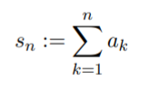
Or, it can be more simply represented by the following summation notation:

Numeric Sequence in Computational Logic
Computational logic uses computers to establish facts in a logical formalism [2]. The facts are defined much more precisely than simple “a sequence of ordered numbers”:
A sequence of characters is a numeric sequence if and only if one of the following is true [3]:
- The sequence is an optionally signed (±) base 10 digit sequence which may or may not have a dot character on the right-hand side.
- The sequence is a #-sequence. A #-sequence has a length of three or more. The first character is always #. The numeric value is the sequence’s base n signed value found by deleting the first two characters. “n” 2, 8, or 16 depending on whether the second character of the sequence is is B, O, or X).
References
[1] Yakir, B. (2011). Introduction to Statistical Thinking (With R, Without Calculus). Retrieved April 3, 2021 from: https://my.uopeople.edu/pluginfile.php/57436/mod_book/chapter/37629/MATH1280.IntroStat.pdf
[2] Proceedings of the Royal Society. Computational logic: its origins and applications. https://royalsocietypublishing.org/doi/10.1098/rspa.2017.0872
[3] Boyer, R. & Moore, S. A Precise Description of a Computational Logic. Retrieved April 3, 2021 from: https://www.cs.utexas.edu/users/boyer/ftp/cs.389r.course.packet.pdf
Random Sequence
A random sequence is a sequence of numbers with zero correlation. In other words, given one number in a sequence {r1, r1, r1, …) there’s no way to predict the second number.
Mathematicians have never been able to agree what is “random” and what isn’t. Many authors have tried (and failed) to pin down a formal definition. Others doubt if such a definition is possible [1]. Every sequence is going to show some kind of pattern or regularity [2].
A Random Sequence Isn’t Really Random
 Some sequence that you think are random actually aren’t at all. For example, if you toss a coin three times, you might think that getting a HHT or TTT or THT is completely random. But that’s not the case, because tossing a coin (assuming it’s a fair one) actually follows the laws of probability: your odds of getting a heads are ½ and your odds of getting a tails are ½.
Computerized “Random Sequence Generators” aren’t truly random either: someone programmed it with a set of deterministic rules that govern what sequence is spat out. Generating a sequence of random number is impossible [3].
What about a human generated random sequence? Off the top of my head, I’m going to type a sequence of random numbers from my laptop keypad (I’ll even keep my eyes closed):
{4578656846879}.
Is this an example of a random sequence? Perhaps surprisingly, the answer is no. Even if you were asked to generate a random sequence of 300 digits between 0 to 9, the result wouldn’t be random either. These types number sequences are not mathematically random; the internal random number generator in your brain is subject to bias, always producing certain patterns [4].
Random Sequence: References
[1] Church, A. On the Concept of Random Sequences. Retrieved 4/9/2021 from: http://www.socsci.uci.edu/~bskyrms/bio/readings/church_randomness.pdf
[2] Random sequences. Retrieved 4/9/2021 from: https://web.northeastern.edu/afeiguin/phys5870/phys5870/node57.html
[3] Volchan, S. What is a Random Sequence? Retrieved 4/9/2021 from: https://www.maa.org/sites/default/files/pdf/upload_library/22/Ford/Volchan46-63.pdf
[4] Schulz, M. et al. (2012) Analysing Humanly Generated Random Number Sequences: A Pattern-Based Approach. Retrieved 4/9/2021 from: https://journals.plos.org/plosone/article?id=10.1371/journal.pone.0041531
Recursive Definition of a Sequence
The word “recursive” means to recur or repeat. In mathematics, it’s the repeated application of a function or rule to successive results. A recursive definition of a sequence defines terms by previous entries in the sequence. It takes the rule for the sequence and applies it over and over, starting with the first term. For example:
- A0 = 0
- An + 1 = An + n + 1
The first term A0 is defined explicitly, as zero. This is the starting point— you need this to build a recursive definition. Every subsequent term in the sequence is defined recursively in terms of An. In other words, you need two parts for a recursive definition of a sequence:
- The initial term (e.g. A0 = 0),
- A recurrence relation (also called a recursion formula): a symbolic description of subsequent terms (e.g. An + 1 = An + n + 1).
The other way to define sequences is with a general term, also called an explicit definition. For example, the sequence defined by an = 1/n only requires you to plug in a value for n. You do not need to know the initial term in order to solve the sequence.
Recursive Definition of a Sequence: Examples
The following sequence is defined recursively with an initial term and a rule for subsequent terms:
- A0 = 3
- An + 1 = An + 5.
The first few terms of the sequence are:
- A0 = 3,
- A1 = A0 + 5 = 3 + 5 = 8,
- A2 = A1 + 5 = (3 + 5) + 5 = 13,
- A3 = A2 + 5 = [(3 + 5) + 5] + 5 = 18,
- A4 = A3 + 5 = {[(3 + 5) + 5] + 5} + 5 = 23.
How to Find the Explicit Definition from a Recursive Definition of a Sequence
There isn’t a formula you can follow to turn a recursive definition to an explicit definition of a sequence. However, there are a few general steps that you can use to identify the pattern needed for an explicit definition.
Step 1: Write out the first few terms of the sequence using the recursive definition, without actually carrying out the arithmetic operations. Using the example above:
- A0 = 3,
- A1 = A0 + 5 = 3 + 5,
- A2 = A1 + 5 = (3 + 5) + 5,
- A3 = A2 + 5 = [(3 + 5) + 5] + 5,
- A4 = A3 + 5 = {[(3 + 5) + 5] + 5} + 5.
Step 2: Look for ways to combine terms. A quick glance at the above terms tells us that 5 is repeating, so we can combine them to get:
- A0 = 3,
- A1 = A0 + 5 = 3 + 5
- A2 = A1 + 5 = 3 + 2(5),
- A3 = A2 + 5 = 3 + 3(5),
- A4 = A3 + 5 = 3 + 4(5).
From here, we can see a pattern emerge: each step in the process multiplies 5 by the term’s index (the index is the subscript in An). For example, the third (A3) has 3 * 5. That leads to the general formula:
an = 3 + 5n.
Recursive Definition of a Sequence: References
Lameda, B. & Nikolaev, N. (2016). Integral Calculus. Retrieved February 4, 2021 from: http://www.math.toronto.edu/beatriz/files/MAT137/MAT136_Lecture_Notes.pdf
What is a Recamán sequence?
There are two different sequences attributed to Columbian puzzle maker Bernardo Recamán Santos:
Recamán sequence #1 (entry A5132 in the OEIS) is usually the one referred to as “The” Recamán Sequence. It is defined by [1]:
- an = an-1 – n, if an-1 – n > 0 and an-1 has already occurred in the sequence.
- Otherwise, an = an-1 + n.
The first few numbers are:
{1, 3, 6, 2, 7, 13, 20, …}.
Recamán sequence #2 (entry A8336 in the OEIS) is defined by:
- an+1 = an / n if n divides an
The first few numbers are:
{1, 1, 2, 6, 24, 120, …}.
Intuitive way to Create the Terms of the Recamán Sequence
Neil Sloane of ATT Labs (creator of OEIS) shed a little light on how the sequence is created in a 2008 Math Factor podcast [2].
Step 1: Write down the numbers
1 2 3 4 5 6 7 8 9
with gaps (we’re going to write the terms in those gaps).
Step 2: Write down the first term, which is 1, between the 1 and the 2:
1 (1) 2 3 4 5 6 7 8 9.
Step 2: Calculate the second term.
Ask yourself the question: Can we subtract 2 (the second number in our list) from 1 (the first term)?. We can’t (negative numbers or zero are not allowed), so we have to add 2 instead. 2 + 1 = 3, so:
1 (1) 2 (3) 3 4 5 6 7 8 9.
Step 2: Calculate the third term in the same way.
Ask yourself the question: Can we subtract 3 (the third number in our list from 3 (the second term). We can’t, so we have to add: 3 + 3 = 6, so:
1 (1) 2 (3) 3 (6) 4 5 6 7 8 9.
Continue in this way, obeying the basic rules:
Numbers can’t be zero, negative, or something already in the sequence.
If any of these conditions appear, just add instead of subtract. Note that if you add and get a number that has appeared before, that’s OK. It’s only not allowed if you subtract.
Deciphering Recaman’s sequence
Although 10230 terms of Recaman’s sequence have been computed, but it still remains a mystery [2] despite the OEIS’s calculation of an enormous number of terms. No one knows if every number will eventually appear; Those dedicated to deciphering the sequence have dubbed it “How to Recamán’s life” [3].
As of the January 2018, Prime Curious! reported that the smallest missing prime in the Sequence is 966727 (as of January 2018).
Random Sequence: References
[1] Ding, C. (2012). Sequences and Their Applications. Springer London.
[2] Math Factor Podcast. Retrieved April 9, 2021 from: http://mathfactor.uark.edu/2008/05/dw-the-online-encyclopedia-of-integer-sequences/
[2] Myers, J. et al. (2020). Three Cousins of Recaman’s Sequence. Retrieved April 9, 2021 from: https://ui.adsabs.harvard.edu/abs/2020arXiv200414000M/abstract
[3] Roberts, S. (2015). Genius At Play: The Curious Mind of John Horton Conway. Bloomsbury Publishing.
Sequence and Series: What is a Series?
A series is what you get when you add up the terms in a sequence; when you add these terms, you’re performing what’s more formally called a summation (which is just a fancy way of saying “add them all up”).
Finite Series
A finite series is a sum of a set amount of terms; A series of numbers (e.g. 1 + 2 + 3) is obtained from a sequence of numbers (e.g. 1, 2, 3); Finite series always have a first term and a last term. Plus, you can always find a solution for the sum of a finite series. For example, you can add up a given series of numbers (like 1 + 2 + 3 + 4) and find the answer (10).
A finite series and infinite series only differ from each other in terms of length. You can think of an infinite series as a “… huge or enormously long series” (Lazerowitz & Ambrose, 2016).
More formally, a finite series has the form (Dragomir & Sofo, 2008):

Where:
- Σ means to “sum up” (called sigma notation),
- ai; i = 1, 2, …, n) is a sequence of numbers.
Finite Series Example: Finite Arithmetic Series
As a slightly more complicated example, the sum of the numbers 1 through 1000 is a finite sum: 500500:
![]()
This particular series is an example of an arithmetic series, which are defined by a common difference between each term (in this example, the difference is 1).
Finite Series Formulas
Some of the more common you’ll come across (Sathaye, 2020):
| Name | |
| Arithmetic Series |  |
| Geometric Series |  |
| Telescoping Series |  |
What is the Dirichlet Series?
The Dirichlet series has the form [1]:

Where:
- s is a real-valued [2] or complex variable (Dirichlet proposed that s should be real or complex, but Riemann later on stressed the importance of s as a complex variable) [3].
- f(n) is a number theoretic function.
The notation s is a long standing tradition (going back to Dirichlet) and is written as s = σ + it, where s is the real part and t is the imaginary part. When σ > 1, the series converges absolutely and serves as a generating function for f(n).
There are hundreds of thousands of infinite and finite Dirichlet series of all kinds [2]. Two of the most well known are the Riemann zeta function, defined as the Dirichlet series associated with the constant function 1, and Dirichlet L-functions [3].
Use of the Dirichlet Series
The series is often seen as a component for many generating functions for arithmetic functions. The method of generating functions is a powerful way of dealing with arithmetic functions. One type of generating functions is a type of power series:
f(0) + f(1)x + f(2)x2…,.
The other type is the Dirichlet series:
![]()
The basic idea is that you relate the function f to the series F [3].
The Dirichlet series is a major component in proofs of the prime number theorem. For example, Hadamard and de la Vallee Poussin developed the first proof of the theorem by using the series to investigate the behavior of partial sums of arithmetic functions; Most proofs of the theorem relate the partial sums
![]()
to a complex integral involving the series
![]()
The integrals are then evaluated with analytic techniques [4].
Dirichlet Series: References
[1] McCarthy, J. (2018). Dirichlet Series, Retrieved December 2, 2020 from: https://www.math.wustl.edu/~mccarthy/amaster-ds.pdf
[2] Gould, H. & Shonhiwa, T. A Catalog of Interesting Dirichlet Series. Retrieved May 4, 2021 from: https://projecteuclid.org/journalArticle/Download?urlid=10.35834%2Fmjms%2F1316032830
[3] Borcherds, R. (2021). Theory of Numbers: Dirichlet Series. https://youtu.be/dTQw2zt2YVw
[4] Hildebrand, A. (2005). Introduction to Analytic Number Theory. Math 531 Lecture Notes, Fall. Retrieved May 4, 2021 from: https://faculty.math.illinois.edu/~hildebr/ant/main4.pdf
Continuous and Discrete Series
The term “continuous series” is used informally, so there isn’t a single definition. Depending on the author, it might mean:
- A series with no breaks,
- As a synonym for an infinite series,
- Where frequencies are given with the variable value (as class intervals).
You’ll want to read up on the authors intention before deciding on an exact definition.
1. A Continuous Series with No Breaks & Discrete Series
A continuous series can be defined as one with has no break or gap in the series. For example, a line segment from two points a to b is the set of all of points between a and b.

Another example: the class of all points (x, y) in a square (including boundaries), arranged in order of magnitude of the x’s (Huntingdon, 2017).
Using the same logic, a discrete series has definite gaps or breaks in between one point and the next. For example, 1, 3, 5, 7,…19 (Singh, 2008).
When used in this sense, what we’re really talking about here is a string of continuous variables (rather than a “continuous series”).
2. Continuous Series with Class Intervals
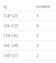
In this definition (sometimes found in statistics and economics), data is divided into continuous groups. It’s similar to the definition in #1 above, except that the groups are placed into a frequency distribution table.
3. Synonym for Infinite Series
Another definition is simply as another name for “infinite series“. For example, in their article The continuous series of critical points of the two-matrix model at N → ∞ in the double scaling limit, Balaska et al. clearly means infinity (because of the → ∞) in the title. In their 1974 book, The Fractional Calculus Theory and Applications of Differentiation and Integration to Arbitrary Order, Keith Oldham and Jerome Spanier mention “…a continuous series of continuously differentiable functions,” which likely falls into the realm of this particular definition.
Stationary Sequence
A real-valued process is a stationary sequence (also called a stationary stochastic process) is defined as one where the following formula is true for every k and m [1]:
![]()
In other words, it is a sequence of random variables that, when shifted, results in the same probability distribution [2]. Informally, you can think of a stationary sequence as modeling successive states of a system in equilibrium [3].
An independent identically distributed (iid) sequence is a special case of a stationary sequence; Stationary is a stronger condition than iid [5].
Strictly and Weakly Stationary Sequence
A sequence is strictly stationary if all n-dimensional distributions of x(t1 + τ),…x(tn + τ) are independent of τ (t is the time lag). A sequence is weakly stationary (or second order stationary) if [4]:
- The mean of the sequence is constant, and
- It’s covariance is function only of the time lag, t.
Ergodic Stationary Sequence
A stationary sequence is ergodic if it satisfies the strong law of large numbers [6]. With a stationary sequence, we’re only concerned with statistical properties (i.e. that a shifted sequence has the same distribution as the original sequence). With ergodicity, we’re concerned with experimental results, or what you actually observe. A stationary process doesn’t have to be ergodic, but the easiest stationary sequences to work with are, because the theoretical distribution will match your experimental results.
Stationary Sequence: References
[1] Roch, S. (2012). Lecture 13 : Stationary Stochastic Processes. Retrieved April 9, 2021 from: https://www.math.wisc.edu/~roch/teaching_files/275b.1.12w/lect13-web.pdf
[2] Hough, B. (2017). Math 639: Lecture
[3] Fristedt, B. & Gray, L. (1997) Stationary Sequences. In A Modern Approach to Probability Theory. pp 553-578. Springer.
[4] Lindgren, G. Lectures on Stationary Stochastic Processes. Retrieved April 9, 2021 from: http://www.maths.lth.se/matstat/staff/georg/Publications/lecture2006.pdf
[5] Sigman, K. (2014). 1 Stationary sequences and Birkhoff ’s Ergodic Theorem. Retrieved April 9, 2021 from: http://www.columbia.edu/~ks20/6712-14/6712-14-Notes-Ergodic.pdf
[6] Appendix A Ergodicity, Martingales, Mixing. Retrieved April 9, 2021 from: https://onlinelibrary.wiley.com/doi/pdf/10.1002/9780470670057.app1
What is a Universal Sequence?
In mathematics, a universal sequence can generate any sequence, within certain bounds. Simply put, it’s a sequence of integers with certain properties.
A universal sequence predictor does exist (at least in theory), which can learn to predict any sequence in existence in the universe. However, the predictor requires too much computing time to be implemented in real life. [4] Because of this impracticality, definitions are normally strictly defined for specific purposes. The exact definition depends on what area of math you’re working with.
For example, a universal sequence for a group is a sequence of words (w1, w2, …) with the following property: The equations wn = sn (where n is a natural number) for any sequence in the group can be solved simultaneously from within the same group [1].
Another example, this time from number theory, which chiefly revolves around the ring of integers (ℤ). ℤ/nℤ, is obtained from universal sequence and has been used to solve an open problem concerning the existence of balanced Steinhaus triangles modulo a positive integer n [2].
Universal Sequence in Chemistry
In chemistry, a recent use of the term comes from Russian researchers Zahed Allahyari and Artem Oganov, who developed a new method for ordering elements of the periodic table. The universal sequence uses radii for atoms and electronegativity to make predictions about basic compounds [3].
Universal Sequence: References
[1] Hyde, J. et al. (2020). Sets of universal sequences for the symmetric group and analogous semigroups. Proc. Amer. Math. Soc. 148. Retrieved April 3, 2021 from: https://www.ams.org/journals/proc/2020-148-05/S0002-9939-2020-14881-2/
[2] Jonathan Chappelon. A universal sequence of integers generating balanced Steinhaus figures modulo an odd number. Journal of Combinatorial Theory, Series A, Elsevier, 2011, 118 (1), pp.291-315. ⟨10.1016/j.jcta.2010.06.005⟩. ⟨hal-00409604v2⟩
[3] Z Allahyari and A R Oganov, (2020). Nonempirical Definition of the Mendeleev Numbers: Organizing the Chemical Space. J. Phys. Chem. C, 2020, 124, 23867 (DOI: 10.1021/acs.jpcc.0c07857)
[4] Hibbard, B. Adversarial Sequence Prediction. Retrieved April 4, 2020 from: https://www.ssec.wisc.edu/~billh/g/hibbard_agi.pdf
Asymptotic Series / Poincaré Expansion
An asymptotic series (also called an asymptotic expansion or Poincaré expansion) is a way of investigating the general behavior of a function as the independent variable (e.g. x) becomes very large. The procedure, which truncates (cuts off) a function after a certain number of terms (a method of partial sums), can get very good approximations with relatively few calculations — especially when the calculations are so complex it would overwhelm most computers (Beckenbach, 2013).
One of the simplest ways to get an asymptotic series is to do a change of variable x→ 1/x, then perform a series expansion about zero. Other ways to generate these series includes the Euler–Maclaurin summation formula, Integral transforms (e.g. the Laplace transform and Mellin transform) and repeated integration by parts.
As an example, the following expansion can be used to find an approximation for the Riemann zeta function:

Any function smaller that every term in an asymptotic series is subdominant to the series. This means that there isn’t a unique function associated with any particular asymptotic series, but rather one of these series defines an entire class of asymptotically equivalent functions. Theses different asymptotic sequences are called gauges (Paulsen, 2013; Goldstein, 2020).
Sequence and Series: Convergence & Divergence of Asymptotic Series
“One remarkable fact of applied mathematics is the ubiquitous appearance of divergent series, hypocritically renamed asymptotic expansions….The challenge of explaining what an asymptotic expansion is ranks among the outstanding taboo problems of mathematics. —Gian-Carlo Rota, in Indiscrete Thoughts (1997), p. 222″
If you find the formal definitions of asymptotic theory challenging to wrap your head around, you aren’t alone in your confusion. Several prominent authors use the term “asymptotic series” to (incorrectly) describe divergent series (e.g. Dingle, 2013; Gradshteyn & Ryzhik, 2007). In general, while all divergent series are asymptotic series (Cousteix & Mauss, 2007; Erdélyi, 1987), the converse isn’t necessarily true: Asymptotic expansions may or may not be divergent. Therefore, you shouldn’t worry about whether or not a particular asymptotic series will converge or diverge until after you have performed the expansion (Michon, 2020).
Stirling Series
The “classical” Stirling series is defined as (Dominic, 2008):

Where the numbers Bk are the Bernoulli numbers.
The series was formulated by the French mathematician Abraham DeMoivre (1667-1994), based on work by Scottish mathematician James Stirling (1692-1770). Stirling wrote the series with powers of 1/(n + ½) (Gellinas, 2017).
Different Definitions for The Stirling Series
The Stirling series can be defined in several closely related ways. For example, as the asymptotic series for the gamma function:
n! = γ(n + 1) = ∫ x2 e-x dx (x: 0 → ∞).
Alternatively it can be defined as the asymptotic expansion of the factorial function n! (Angelis, 2009):

The series is sometimes defined as an asymptotic expansion of Stirling’s formula, a good approximation for factorials:
log(n!) = n log n −n + ½ log(n) + log √ (2 π) + εn,
Where εn → 0 as n → ∞. It replaces epsilon(ε) with powers of 1/n (Conrad, 2020).
Stirling’s series can also be defined as the following divergent series (Impens, 2003)

Where A, B, C… are positive constants.
Stirling Series: References
Abramowitz, M. & Stegun, I. A. (Eds.) (1972). Handbook of Mathematical Functions with Formulas, Graphs, and Mathematical Tables, 9th printing. New York: Dover, p. 257.
Angelis, V. (2009). Stirling’s Series Revisited. The American Mathematical Monthly
Vol. 116, No. 9 (Nov), pp. 839-843. Taylor & Francis, Ltd.
Arfken, G. (1985). “Stirling’s Series.” §10.3 in Mathematical Methods for Physicists, 3rd ed. Orlando, FL: Academic Press, pp. 555-559.
Conrad, K. (2020). Stirling’s Formula. Retrieved November 20, 2020 from https://kconrad.math.uconn.edu/blurbs/analysis/stirling.pdf
Dominici, D. (2008). Variations on a theme by James Stirling. Note di Matematica
Note Mat. 1.
Ferraro, G. (2008). The Rise and Development of the Theory of Series up to the Early 1820s. Springer.
Gelinas, J. (2017). Original proofs of Stirling’s series for log(n!). Retrieved November 20, 2020 from: https://arxiv.org/abs/1701.06689.
Impens, C. (2003). Stirling’s Series Made Easy. Retrieved November 20, 2020 from: https://cage.ugent.be/~ci/impens_stirling.pdf
Trigonometric Series
Trigonometric Series & Polynomial
A trigonometric series is a series of cosines and sines of multiple angles. This powerful way to represent and study functions has the form (Kechris, 2020):

Where:
- an ∈ ℂ (the complex plane),
- x ∈ ℝ (the reals).
The nth partial sum of the trigonometric series is called the trigonometric polynomial.
The trigonometric series turns into the Fourier series if an and bn (the coefficients of the trigonometric series) have the form:

Where f is an integrable function.
One application of trigonometric sequences and series is to approximate π. For example, an accelerated version of Vieta’s formula
![]()
can approximate π to 300,000 decimal places (Kreminski, 2008).
Theory of Trigonometric Series
The theory of trigonometric series spawned several other important theoretical branches including construction of the Riemann integral and Lebesgue integrals plus several generalizations of the theory, including (Hazelwinkel, 1993):
- Abstract harmonic analysis,
- Almost-periodic functions,
- Fourier integral,
- General orthogonal series.
In addition, the theory of trigonometric series was a starting point for the development of set theory.
Trigonometric Function Series
Although the term “trigonometric series” usually refers to the formula at the top of this article, it may also refer to the expansion of trigonometric functions into their power series. For example: (Nave, 2020).
- sine(x) = x – (x3/3!) + (x5/5!) – (x7/7!)…
- cos(x) = 1 – (x2/2!) + (x4/4!) – (x6/6!)…
- cos(x) = x + (x3/3!) + (2x5/15!) – (17x7/315!)…
Where ! is a factorial.
These expansions can be used to approximate tiny values of x. For example, when the angle x is in radians, small values for sin(x) = x, small cos(x) = 1 and small tan(x) = x.
Trigonometric Series: References
Hazelwinkel, M. (1993). Encyclopaedia of Mathematics: Stochastic Approximation — Zygmund Class of Functions. Springer.
Kechris, A. (2020). Set Theory and Uniqueness for Trigonometric Series. Retrieved November 15, 2020 from: http://www.math.caltech.edu/~kechris/papers/uniqueness.pdf
Kreminski, R. (2008). π to Thousands of Digits from Vieta’s Formula, Mathematics
Magazine 81, No. 3, June, 2008, 201-207.
Nave, R. (2020). Trig Function Series. Retrieved November 15, 2020.
Zygmund, A. (2002). Trig. Series. Cambridge University Press.
Sequence of Functions
A sequence of functions {fn(x)} is a family of functions where “x” (or the parameter set) is a sequence of natural numbers (the counting numbers 1, 2, 3…).
For example, let’s say the sequence of functions was defined by {xn}. Each n will result in a new function:
- x1,
- x2,
- x3,
- …xn.
You can also fix the x to get a numeric sequence; If x = 2 then the formula becomes the geometric sequence {2n [1].
Convergence of Sequence of Functions
If you a working with real-valued functions, a good place to start studying convergence is to graph all of the functions (substituting in 1, 2, 3, … for “n”) to see where they converge.
For example, the sequence of functions f(x) = x/n converges pointwise to the limit function f(x) = 0 for the closed interval [0, 1]:
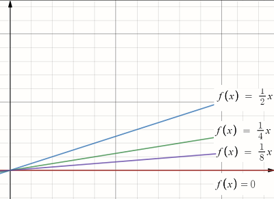
Pointwise convergence is defined as follows [2]:
A sequence {fn} of functions fn: X → ℝ converges pointwise to a function fn: X → ℝ if for every x the sequence of real numbers {fn(x)} converges the number f(x).
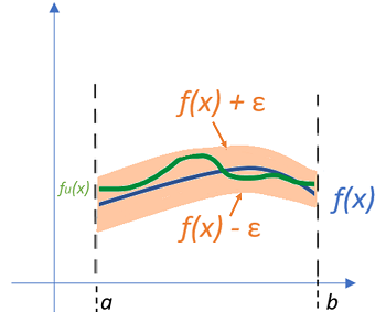
Uniform convergence is defined more strictly than pointwise convergence. Values must stay in a “box” around the function.
Proving Convergence of a Sequence of Functions
Showing that a sequence of functions converges is relatively simple. You can graph the possibilities and see where they converge. Or, plug in a few values in the given interval and see where the functions head that way. Proving that a sequence of functions converges is a little trickier. It’s not difficult, but as it’s a formal proof, it involves a fair amount of terminology like epsilon(ε). The basic idea is that you need to look at the behavior of the sequence at the endpoints and in the middle. You then fill in a formal proof.
The following video may be helpful. It shows a proof for fn0 = xn.
References
[1] Interactive Real Analysis: Sequences of Functions. Retrieved April 3, 2021 from: https://mathcs.org/analysis/reals/funseq/pconv.html
[2] Convergence of Sequences of Functions: Some Additional Notes. Retrieved April 3, 2021 from: http://www.u.arizona.edu/~mwalker/econ519/Econ519LectureNotes/AddlNotesConvergenceOfSequences.pdf
Sequence and Series: Related Articles
- Alternating Series Test
- Pointwise Convergence
- Series Rules
- Remainder of a Series
- Series Convergence Tests
- Sum of a Convergent Geometric Series
Sequence and Series: References
Balaska, S. et al. (1998). The continuous series of critical points of the two-matrix model at N → ∞ in the double scaling limit. Nuclear Physics, Section B, Volume 520, Issue 1, p. 411-432.
Beckenbach, E. (2013). Modern Mathematics for the Engineer: Second Series. Dover Publications.
Caldwell, C. (2020). Arithmetic Sequence. Retrieved August 26, 2020 from: https://primes.utm.edu/glossary/page.php?sort=ArithmeticSequence
Cousteix, J. & Mauss, J. (2017). Asymptotic Analysis and Boundary Layers. Springer.
Dingle, R. (2013). Asymptotic Expansions: Their Derivation and Interpretation. Academic Press.
Dragomir, S. & Sofo, A. (2008). Advances in Inequalities for Series. Nova Science Publishers.
Erdélyi, A. (1987). Asymptotic Expansions. New York: Dover,.
Goldstein, R. (2020). Asymptotic versus Convergent series. Optimal truncation. Retrieved November 22, 2020 from: http://www.damtp.cam.ac.uk/user/gold/pdfs/teaching/L3.pdf
Gradshteyn, S. and Ryzhik, I. (2007). Table of Integrals, Series, and Products. Edited by A. Jeffrey and D. Zwillinger. Academic Press, New York, 7th edition.
Huntingdon, E. (2017). The Continuum and Other Types of Serial Order: Second Edition. Courier Dover Publications.
Lozano-Robledo, A. (2019). Number Theory and Geometry. An Introduction to Arithmetic Geometry. American Mathematical Society.
Larson, R. & Edwards, B. (2013). Calculus. Cengage Learning; 10 editionOldham, K. & Spanier, J. (1974). The Fractional Calculus Theory and Applications of Differentiation and Integration to Arbitrary Order. Elsevier Science.
Lazerowitz, M. & Ambrose, A. (2016). Necessity and Language. Taylor & Francis.
Maor, E. (1991). To Infinity and Beyond. A Cultural History of the Infinite. Princeton University Press.
Michon, G. (2020). Asymptotic Analysis. Retrieved November 20, 2020 from: http://www.numericana.com/answer/asymptotic.htm#series
Paulsen, W. (2013). Asymptotic Analysis and Perturbation Theory. Chapman and Hall/CRC.
Riley, K. et al. (2006). Mathematical Methods for Physics and Engineering. A Comprehensive Guide.
Rota, G. (2000). Indiscrete Thoughts. Birkhäuser.
Sathaye, A. Finite Series Formulas. Retrieved August 9, 2020 from: http://www.msc.uky.edu/sohum/ma110/text/formulas/node2.html
Singh, S. (2008). Biostatistics And Introductory Calculus. Nirali Prakashan.