Contents:
What is a Z Table: Overview

Can’t see the video? Click here to watch it on YouTube.
The z-table is short for the “Standard Normal z-table”. The Standard Normal model is used in hypothesis testing, including tests on proportions and on the difference between two means. The area under the whole of a normal distribution curve is 1, or 100 percent. The z-table helps by telling us what percentage is under the curve at any particular point.
What is a Z Table: Standard Normal Probability
Every set of data has a different set of values. For example, heights of people might range from eighteen inches to eight feet and weights can range from one pound (for a preemie) to five hundred pounds or more. Those wide ranges make it difficult to analyze data, so we “standardize” the normal curve, setting it to have a mean of zero and a standard deviation of one. When the curve is standardized, we can use a Z Table to find percentages under the curve.
Percentages under the curve

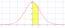
This graph shows the standardized normal graph with the percentage of results (data) that will fall between standard deviations on that graph. For example, 68.27 percent of results will fall within one standard deviation of the mean. On this graph, it’s represented by two z-scores from the z table: the area between z = -1 and z = 1.
The z-table
Obviously a graph can only give us so much information. The above graph can tell us the area under the curve for one (z = -1 to 1), two (z = -2 to 2) and three (z = -3 to 3) standard deviations from the center. But what about if we want to know the area between z = -0.78 and z = 0.78? Or z = -1.2 and z=0.44? That’s where the z-table comes in. It tells us the area under the standard normal curve for any value between the mean (zero) and any z-score.
Why Are There at least Two z-tables?
Simply, it’s to make life easier. Sometimes you’ll want to know the area between the mean and some positive value. That’s when you’ll use the right-hand z-table. But other times you might want to know the area in a left tail. If that’s the case, use the z-table that shows the area to the left of z.
Check out the StatisticsHowTo.com YouTube channel!
Z-Table (right)
This z-table (normal distribution table) shows the area to the right hand side of the curve. Use these values to find the area between z=0 and any positive value. For an area in a left tail, look at this left-tail z-table instead.
| z | 0.00 | 0.01 | 0.02 | 0.03 | 0.04 | 0.05 | 0.06 | 0.07 | 0.08 | 0.09 |
|---|---|---|---|---|---|---|---|---|---|---|
| 0.0 | 0.0000 | 0.0040 | 0.0080 | 0.0120 | 0.0160 | 0.0199 | 0.0239 | 0.0279 | 0.0319 | 0.0359 |
| 0.1 | 0.0398 | 0.0438 | 0.0478 | 0.0517 | 0.0557 | 0.0596 | 0.0636 | 0.0675 | 0.0714 | 0.0753 |
| 0.2 | 0.0793 | 0.0832 | 0.0871 | 0.0910 | 0.0948 | 0.0987 | 0.1026 | 0.1064 | 0.1103 | 0.1141 |
| 0.3 | 0.1179 | 0.1217 | 0.1255 | 0.1293 | 0.1331 | 0.1368 | 0.1406 | 0.1443 | 0.1480 | 0.1517 |
| 0.4 | 0.1554 | 0.1591 | 0.1628 | 0.1664 | 0.1700 | 0.1736 | 0.1772 | 0.1808 | 0.1844 | 0.1879 |
| 0.5 | 0.1915 | 0.1950 | 0.1985 | 0.2019 | 0.2054 | 0.2088 | 0.2123 | 0.2157 | 0.2190 | 0.2224 |
| 0.6 | 0.2257 | 0.2291 | 0.2324 | 0.2357 | 0.2389 | 0.2422 | 0.2454 | 0.2486 | 0.2517 | 0.2549 |
| 0.7 | 0.2580 | 0.2611 | 0.2642 | 0.2673 | 0.2704 | 0.2734 | 0.2764 | 0.2794 | 0.2823 | 0.2852 |
| 0.8 | 0.2881 | 0.2910 | 0.2939 | 0.2967 | 0.2995 | 0.3023 | 0.3051 | 0.3078 | 0.3106 | 0.3133 |
| 0.9 | 0.3159 | 0.3186 | 0.3212 | 0.3238 | 0.3264 | 0.3289 | 0.3315 | 0.3340 | 0.3365 | 0.3389 |
| 1.0 | 0.3413 | 0.3438 | 0.3461 | 0.3485 | 0.3508 | 0.3531 | 0.3554 | 0.3577 | 0.3599 | 0.3621 |
| 1.1 | 0.3643 | 0.3665 | 0.3686 | 0.3708 | 0.3729 | 0.3749 | 0.3770 | 0.3790 | 0.3810 | 0.3830 |
| 1.2 | 0.3849 | 0.3869 | 0.3888 | 0.3907 | 0.3925 | 0.3944 | 0.3962 | 0.3980 | 0.3997 | 0.4015 |
| 1.3 | 0.4032 | 0.4049 | 0.4066 | 0.4082 | 0.4099 | 0.4115 | 0.4131 | 0.4147 | 0.4162 | 0.4177 |
| 1.4 | 0.4192 | 0.4207 | 0.4222 | 0.4236 | 0.4251 | 0.4265 | 0.4279 | 0.4292 | 0.4306 | 0.4319 |
| 1.5 | 0.4332 | 0.4345 | 0.4357 | 0.4370 | 0.4382 | 0.4394 | 0.4406 | 0.4418 | 0.4429 | 0.4441 |
| 1.6 | 0.4452 | 0.4463 | 0.4474 | 0.4484 | 0.4495 | 0.4505 | 0.4515 | 0.4525 | 0.4535 | 0.4545 |
| 1.7 | 0.4554 | 0.4564 | 0.4573 | 0.4582 | 0.4591 | 0.4599 | 0.4608 | 0.4616 | 0.4625 | 0.4633 |
| 1.8 | 0.4641 | 0.4649 | 0.4656 | 0.4664 | 0.4671 | 0.4678 | 0.4686 | 0.4693 | 0.4699 | 0.4706 |
| 1.9 | 0.4713 | 0.4719 | 0.4726 | 0.4732 | 0.4738 | 0.4744 | 0.4750 | 0.4756 | 0.4761 | 0.4767 |
| 2.0 | 0.4772 | 0.4778 | 0.4783 | 0.4788 | 0.4793 | 0.4798 | 0.4803 | 0.4808 | 0.4812 | 0.4817 |
| 2.1 | 0.4821 | 0.4826 | 0.4830 | 0.4834 | 0.4838 | 0.4842 | 0.4846 | 0.4850 | 0.4854 | 0.4857 |
| 2.2 | 0.4861 | 0.4864 | 0.4868 | 0.4871 | 0.4875 | 0.4878 | 0.4881 | 0.4884 | 0.4887 | 0.4890 |
| 2.3 | 0.4893 | 0.4896 | 0.4898 | 0.4901 | 0.4904 | 0.4906 | 0.4909 | 0.4911 | 0.4913 | 0.4916 |
| 2.4 | 0.4918 | 0.4920 | 0.4922 | 0.4925 | 0.4927 | 0.4929 | 0.4931 | 0.4932 | 0.4934 | 0.4936 |
| 2.5 | 0.4938 | 0.4940 | 0.4941 | 0.4943 | 0.4945 | 0.4946 | 0.4948 | 0.4949 | 0.4951 | 0.4952 |
| 2.6 | 0.4953 | 0.4955 | 0.4956 | 0.4957 | 0.4959 | 0.4960 | 0.4961 | 0.4962 | 0.4963 | 0.4964 |
| 2.7 | 0.4965 | 0.4966 | 0.4967 | 0.4968 | 0.4969 | 0.4970 | 0.4971 | 0.4972 | 0.4973 | 0.4974 |
| 2.8 | 0.4974 | 0.4975 | 0.4976 | 0.4977 | 0.4977 | 0.4978 | 0.4979 | 0.4979 | 0.4980 | 0.4981 |
| 2.9 | 0.4981 | 0.4982 | 0.4982 | 0.4983 | 0.4984 | 0.4984 | 0.4985 | 0.4985 | 0.4986 | 0.4986 |
| 3.0 | 0.4987 | 0.4987 | 0.4987 | 0.4988 | 0.4988 | 0.4989 | 0.4989 | 0.4989 | 0.4990 | 0.4990 |
| 3.1 | 0.4990 | 0.4991 | 0.4991 | 0.4991 | 0.4992 | 0.4992 | 0.4992 | 0.4992 | 0.4993 | 0.4993 |
| 3.2 | 0.4993 | 0.4993 | 0.4994 | 0.4994 | 0.4994 | 0.4994 | 0.4994 | 0.4995 | 0.4995 | 0.4995 |
| 3.3 | 0.4995 | 0.4995 | 0.4995 | 0.4996 | 0.4996 | 0.4996 | 0.4996 | 0.4996 | 0.4996 | 0.4997 |
| 3.4 | 0.4997 | 0.4997 | 0.4997 | 0.4997 | 0.4997 | 0.4997 | 0.4997 | 0.4997 | 0.4997 | 0.4998 |
| 3.5 | 0.4998 | 0.4998 | 0.4998 | 0.4998 | 0.4998 | 0.4998 | 0.4998 | 0.4998 | 0.4998 | 0.4998 |
| 3.6 | 0.4998 | 0.4998 | 0.4999 | 0.4999 | 0.4999 | 0.4999 | 0.4999 | 0.4999 | 0.4999 | 0.4999 |
| 3.7 | 0.4999 | 0.4999 | 0.4999 | 0.4999 | 0.4999 | 0.4999 | 0.4999 | 0.4999 | 0.4999 | 0.4999 |
| 3.8 | 0.4999 | 0.4999 | 0.4999 | 0.4999 | 0.4999 | 0.4999 | 0.4999 | 0.4999 | 0.4999 | 0.4999 |
Left Z-Table
This table shows the area to the left of Z. In other words, the area of a left hand tail. If you want to find the value between z=0 and a positive number, use the right-hand z-table (above) instead (Hint: if you’re asked to look at the “z-table”, in most cases you’ll want to be looking at the other z-table!)
| Z | 0.00 | 0.01 | 0.02 | 0.03 | 0.04 | 0.05 | 0.06 | 0.07 | 0.08 | 0.09 |
|---|---|---|---|---|---|---|---|---|---|---|
| 0.0 | 0.5000 | 0.5040 | 0.5080 | 0.5120 | 0.5160 | 0.5199 | 0.5239 | 0.5279 | 0.5319 | 0.5359 |
| 0.1 | 0.5398 | 0.5438 | 0.5478 | 0.5517 | 0.5557 | 0.5596 | 0.5636 | 0.5675 | 0.5714 | 0.5753 |
| 0.2 | 0.5793 | 0.5832 | 0.5871 | 0.5910 | 0.5948 | 0.5987 | 0.6064 | 0.1064 | 0.6103 | 0.6141 |
| 0.3 | 0.6179 | 0.6217 | 0.6255 | 0.6293 | 0.6331 | 0.6368 | 0.6406 | 0.6443 | 0.6480 | 0.6517 |
| 0.4 | 0.6554 | 0.6591 | 0.6628 | 0.6664 | 0.6700 | 0.6736 | 0.6772 | 0.6808 | 0.6844 | 0.6879 |
| 0.5 | 0.6915 | 0.6950 | 0.6985 | 0.7019 | 0.7054 | 0.7088 | 0.7123 | 0.7157 | 0.7190 | 0.7224 |
| 0.6 | 0.7257 | 0.7291 | 0.7324 | 0.7357 | 0.7389 | 0.7422 | 0.7454 | 0.7486 | 0.7517 | 0.7549 |
| 0.7 | 0.7580 | 0.7611 | 0.7642 | 0.7673 | 0.7704 | 0.7734 | 0.7764 | 0.7794 | 0.7823 | 0.7852 |
| 0.8 | 0.7881 | 0.7910 | 0.7939 | 0.7967 | 0.7995 | 0.8023 | 0.8051 | 0.8078 | 0.8106 | 0.8133 |
| 0.9 | 0.8159 | 0.8186 | 0.8212 | 0.8238 | 0.8264 | 0.8289 | 0.8315 | 0.8340 | 0.8365 | 0.8389 |
| 1.0 | 0.8413 | 0.8438 | 0.8461 | 0.8485 | 0.8508 | 0.8531 | 0.8554 | 0.8577 | 0.8599 | 0.8621 |
| 1.1 | 0.8643 | 0.8665 | 0.8686 | 0.8708 | 0.8729 | 0.8749 | 0.8770 | 0.8790 | 0.8810 | 0.8830 |
| 1.2 | 0.8849 | 0.8869 | 0.8888 | 0.8907 | 0.8925 | 0.8944 | 0.8962 | 0.8980 | 0.8997 | 0.9015 |
| 1.3 | 0.9032 | 0.9049 | 0.9066 | 0.9082 | 0.9099 | 0.9115 | 0.9131 | 0.9147 | 0.9162 | 0.9177 |
| 1.4 | 0.9192 | 0.9207 | 0.9222 | 0.9236 | 0.9251 | 0.9265 | 0.9279 | 0.9292 | 0.9306 | 0.9319 |
| 1.5 | 0.9332 | 0.9345 | 0.9357 | 0.9370 | 0.9382 | 0.9394 | 0.9406 | 0.9418 | 0.9429 | 0.9441 |
| 1.6 | 0.9452 | 0.9463 | 0.9474 | 0.9484 | 0.9495 | 0.9505 | 0.9515 | 0.9525 | 0.9535 | 0.9545 |
| 1.7 | 0.9554 | 0.9564 | 0.9573 | 0.9582 | 0.9591 | 0.9599 | 0.9608 | 0.9616 | 0.9625 | 0.9633 |
| 1.8 | 0.9641 | 0.9649 | 0.9656 | 0.9664 | 0.9671 | 0.9678 | 0.9686 | 0.9693 | 0.9699 | 0.9706 |
| 1.9 | 0.9713 | 0.9719 | 0.9726 | 0.9732 | 0.9738 | 0.9744 | 0.9750 | 0.9756 | 0.9761 | 0.9767 |
| 2.0 | 0.9772 | 0.9778 | 0.9783 | 0.9788 | 0.9793 | 0.9798 | 0.9803 | 0.9808 | 0.9812 | 0.9817 |
| 2.1 | 0.9821 | 0.9826 | 0.9830 | 0.9834 | 0.9838 | 0.9842 | 0.9846 | 0.9850 | 0.9854 | 0.9857 |
| 2.2 | 0.9861 | 0.9864 | 0.9868 | 0.9871 | 0.9875 | 0.9878 | 0.9881 | 0.9884 | 0.9887 | 0.9890 |
| 2.3 | 0.9893 | 0.9896 | 0.9898 | 0.9901 | 0.9904 | 0.9906 | 0.9909 | 0.9911 | 0.9913 | 0.9916 |
| 2.4 | 0.9918 | 0.9920 | 0.9922 | 0.9925 | 0.9927 | 0.9929 | 0.9931 | 0.9932 | 0.9934 | 0.9936 |
| 2.5 | 0.9938 | 0.9940 | 0.9941 | 0.9943 | 0.9945 | 0.9946 | 0.9948 | 0.9949 | 0.9951 | 0.9952 |
| 2.6 | 0.9953 | 0.9955 | 0.9956 | 0.9957 | 0.9959 | 0.9960 | 0.9961 | 0.9962 | 0.9963 | 0.9964 |
| 2.7 | 0.9965 | 0.9966 | 0.9967 | 0.9968 | 0.9969 | 0.9970 | 0.9971 | 0.9972 | 0.9973 | 0.9974 |
| 2.8 | 0.9974 | 0.9975 | 0.9976 | 0.9977 | 0.9977 | 0.9978 | 0.9979 | 0.9979 | 0.9980 | 0.9981 |
| 2.9 | 0.9981 | 0.9982 | 0.9982 | 0.9983 | 0.9984 | 0.9984 | 0.9985 | 0.9985 | 0.9986 | 0.9986 |
| 3.0 | 0.9987 | 0.9987 | 0.9987 | 0.9988 | 0.9988 | 0.9989 | 0.9989 | 0.9989 | 0.9990 | 0.9990 |
References
Beyer, W. (2017). Handbook of Tables for Probability and Statistics 2nd Edition. CRC Press.