Statistics Definitions > Convergence of random variables
Contents:
- What is convergence of random variables?
- Convergence in probability,
- Convergence in distribution,
- Almost sure convergence,
- Convergence in mean.
- Absolutely & Conditionally Convergent
- Positive Terms Series
- Series with Positive and Negative Terms
- Conditional Convergence and the Riemann Series Theorem
- Pointwise Convergence
- Uniform Convergence
- Rate of Convergence
What is convergence of random variables?
Convergence of random variables (sometimes called stochastic convergence) is where a set of numbers settle on a particular number. It works the same way as convergence in everyday life; For example, cars on a 5-line highway might converge to one specific lane if there’s an accident closing down four of the other lanes. In the same way, a sequence of numbers (which could represent cars or anything else) can converge (mathematically, this time) on a single, specific number. Certain processes, distributions and events can result in convergence— which basically mean the values will get closer and closer together.
When Random variables converge on a single number, they may not settle exactly that number, but they come very, very close. In notation, x (xn → x) tells us that a sequence of random variables (xn) converges to the value x. This is only true if the https://www.statisticshowto.com/absolute-value-function/#absolute of the differences approaches zero as n becomes infinitely larger. In notation, that’s:
|xn − x| → 0 as n → ∞.
What happens to these variables as they converge can’t be crunched into a single definition. Instead, several different ways of describing the behavior are used.
Convergence of Random Variables can be broken down into many types. Each of these definitions is quite different from the others. However, for an infinite series of independent random variables: convergence in probability, convergence in distribution, and almost sure convergence are equivalent [1].
1. Convergence in probability
If you toss a coin n times, you would expect heads around 50% of the time. However, let’s say you toss the coin 10 times. You might get 7 tails and 3 heads (70%), 2 tails and 8 heads (20%), or a wide variety of other possible combinations. Eventually though, if you toss the coin enough times (say, 1,000), you’ll probably end up with about 50% tails. In other words, the percentage of heads will converge to the expected probability.
More formally, convergence in probability can be stated as the following formula:
![]()
Where:
- P = probability,
- Xn = number of observed successes (e.g. tails) in n trials (e.g. tosses of the coin),
- Lim (n→∞) = the limit at infinity — a number where the distribution converges to after an infinite number of trials (e.g. tosses of the coin),
- c = a constant where the sequence of random variables converge in probability to,
- ε = a positive number representing the distance between the expected value and the observed value.
The concept of a limit is important here; in the limiting process, elements of a sequence become closer to each other as n increases. In simple terms, you can say that they converge to a single number.
2. Convergence in distribution
Convergence in distribution (sometimes called convergence in law) is based on the distribution of random variables, rather than the individual variables themselves. It is the convergence of a sequence of cumulative distribution functions (CDF). As it’s the CDFs, and not the individual variables that converge, the variables can have different probability spaces.
In more formal terms, a sequence of random variables converges in distribution if the CDFs for that sequence converge into a single CDF. Let’s say you had a series of random variables, Xn. Each of these variables X1, X2,…Xn has a CDF FXn(x), which gives us a series of CDFs {FXn(x)}. Convergence in distribution implies that the CDFs converge to a single CDF, Fx(x) [2].
Several methods are available for proving convergence in distribution. For example, Slutsky’s Theorem and the Delta Method can both help to establish convergence. Convergence of moment generating functions can prove convergence in distribution, but the converse isn’t true: lack of converging MGFs does not indicate lack of convergence in distribution. Scheffe’s Theorem is another alternative, which is stated as follows [3]:
Let’s say that a sequence of random variables Xn has probability mass function (PMF) fn and each random variable X has a PMF f. If it’s true that fn(x) → f(x) (for all x), then this implies convergence in distribution. Similarly, suppose that Xn has cumulative distribution function (CDF) fn (n ≥ 1) and X has CDF f. If it’s true that fn(x) → f(x) (for all but a countable number of X), that also implies convergence in distribution.
3. Almost sure (a.s.) convergence
Almost sure convergence (also called convergence in probability one) answers the question: given a random variable X, do the outcomes of the sequence Xn converge to the outcomes of X with a probability of 1? [4].
As an example of this type of convergence of random variables, let’s say an entomologist is studying feeding habits for wild house mice and records the amount of food consumed per day. The amount of food consumed will vary wildly, but we can be almost sure (quite certain) that amount will eventually become zero when the animal dies. It will almost certainly stay zero after that point. We’re “almost certain” because the animal could be revived, or appear dead for a while, or a scientist could discover the secret for eternal mouse life. In life — as in probability and statistics — nothing is certain.
Almost sure convergence is defined in terms of a scalar sequence or matrix sequence:
- Scalar: Xn has almost sure convergence to X iff: P|Xn → X| = P(limn→∞Xn = X) = 1
- Matrix: Xn has almost sure convergence to X iff: P|yn[i,j] → y[i,j]| = P(limn→∞yn[i,j] = y[i,j]) = 1, for all i and j.
Almost Sure in Convergence vs. Convergence in Probability
The difference between almost sure convergence (called strong consistency for b) and convergence in probability (called weak consistency for b) is subtle. It’s what Cameron and Trivedi [4] call “…conceptually more difficult” to grasp. The main difference is that convergence in probability allows for more erratic behavior of random variables. You can think of it as a stronger type of convergence, almost like a stronger magnet, pulling the random variables in together. If a sequence shows almost sure convergence (which is strong), that implies convergence in probability (which is weaker). The converse is not true — convergence in probability does not imply almost sure convergence, as the latter requires a stronger sense of convergence.
4. Convergence in mean.
A series of random variables Xn converges in mean of order p to X if:
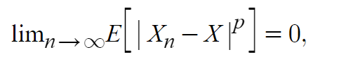
Where 1 ≤ p ≤ ∞.
When p = 1, it is called convergence in mean (or convergence in the first mean). When p = 2, it’s called mean-square convergence.
Convergence in mean is stronger than convergence in probability (this can be proved by using Markov’s Inequality). Although convergence in mean implies convergence in probability, the reverse is not true.
Absolutely & Conditionally Convergent
Although you can generally say that something converges if it settles on a number, convergence in calculus (or calculus based statistics) is usually defined more strictly, depending on whether the convergence is conditional or absolute.
A series is absolutely convergent if the series converges and it also converges when all terms in the series are replaced by their absolute values.
Conditional Convergence is a special kind of convergence where a series is convergent when seen as a whole, but the absolute values diverge. It’s sometimes called semi-convergent.
A series is absolutely convergent if the series converges (approaches a certain number) and it also converges when all terms in the series are replaced by their absolute values. In other words,
…if |u1| + |u2| +… is convergent, then the series u1 + u2 +… is absolutely convergent.
This statement is usually written with the summation symbol:
if Σ |un| is convergent, then the series Σ un has absolute convergence.
Positive Terms Series
If the series of positive terms converges, then both the series of positive terms and the alternating series (i.e. a series with alternating positive and negative terms) will converge.
If a convergent series is a set of positive terms, then that series is also absolutely convergent. That’s because Σun and Σ|un| are the same series.
Series with Positive and Negative Terms
If a convergent series has an infinite number of positive terms and an infinite number of negative terms, it only has absolute convergence if Σ|un is also convergent.
Conditional Convergence and the Riemann Series Theorem
As stated above, conditional convergence is a special kind of convergence where a series is convergent (i.e. settles on a certain number) when seen as a whole. However, there’s a catch:
- The sum of its positive terms goes to positive infinity and
- The sum of its negative terms goes to negative infinity.
It has a very special property, called the Riemann series theorem, that says that it can be made to converge to any desired value—or to diverge—by simple rearrangement of the terms.
In order to find out if a series is conditionally convergent:
- Find out if the series converges, then
- Determine it isn’t absolutely convergent:
- The Alternating series test tells us that if the terms of the series alternates in sign (e.g. -x, +x, -x…), and each term is bigger than the term after it, the series converges.
- Take the absolute values of the alternating (converging) series. If the new (all positive term) series converges, then the series is absolutely convergent. If that new series is not convergent, the original series was only conditionally convergent.
The Riemann Series Theorem
It might seem counter-intuitive that a series can be made to converge to anything just by rearranging the terms. But if you have a well-defined limit you want it to approach, all you need to do is:
- Take enough positive terms to just barely exceed the desired limit, then
- Add enough negative terms to go below the desired limit, then
Continue in this way.
Since all terms of the original series go to zero, the new, rearranged series will converge to the limit you chose.
As an example of the Riemann series consider the alternating harmonic series. As written, it converges to ln2. But can we make it converge to half of that, (ln2)/2. The ordinary way, it would be written
1 – 1/2 + 1/3 – 1/4 +….
Every other term is negative. But if we arrange it as (one positive term) + (two negative terms), we get this:
1 – 1/2 -1/4 + 1/3…
We can rewrite this as:
(1 – 1/2) + (1/3 – 1/4 – 1/6) + (1/5 – 1/8 – 1/10) + …
Which is one half of what the original series converged to.
Pointwise Convergence
Pointwise convergence is where a sequence of functions converges onto a single function, called a limiting function (or limit function). A sequence of functions, denoted { fn(x) }, is a family of functions with a parameter set of natural numbers (whole, non-negative numbers that we use to count like 1, 2, 3,…).
For example, the sequence of functions f(x) = x/n converges to the limiting function f(x) = 0 for the closed interval [0, 1], as shown in the following image:
Compared to uniform Convergence, this is a fairly simple type of convergence. One of the main differences between the two types of convergence is that the limiting function of a pointwise convergent sequence doesn’t have to be a continuous function, while a limiting function of a uniformly convergent sequence does have to be continuous.
As pointwise convergence is a relatively simple way to define convergence for a sequence of functions, you may be wondering why a formal definition is even needed. Although convergence seems to happen naturally (like the sequence of functions f(x) = x/n shown above), not all functions are so well behaved. In order to show that a series of functions has pointwise convergence, you must prove that it meets the formal definition. That said, the definition is fairly straightforward:
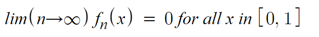
A sequence of functions fn shows pointwise convergence for a set A if the following holds for all x ∈ A:
lim(n→∞) fn(x) = f(x)
Uniform Convergence
Uniform convergence is where a series of continuous functions converges on one particular function f(x), called the limiting function. This type of convergence is defined more strictly than pointwise convergence. The idea of uniform convergence is very similar to uniform continuity, where values must stay inside a defined “box” around the function.
As an example, the series f(x) = x/n converges to f(x) = 0 on the closed interval [0, 1]:
This series of functions uniformly converges to f(x) = 0, called the limiting function.
Note how the slope of each function gets lower and lower, eventually converging on f(x) = 0 (which is essentially, a function that goes along the x-axis).
Although these functions are converging on a limiting function (f(x) = 0, in the above example), the sequence may or may not be converging uniformly to that function. Uniform convergence is a particular type of convergence where the limiting function must be within a set “boundary” around two values: between two tiny values (“epsilon“):-ε and ε.
Formal Definition of Uniform Convergence
A sequence of real-valued continuous functions (f1, f2…fn), defined on a closed interval [a, b], has uniform convergence if the following inequality is true for all x in the domain:
|fn(x) – f(x)| < ε for all x ∈ D whenever n ≥ N, Where:
- N = a positive integer that only depends on ε,
- D = the domain,
- ∈ = “is an element of” (i.e. “is in the set”)
Pointwise Convergence vs. Uniform Convergence
If a function is uniformly convergent, then it is also pointwise convergent to the same limit (but note that this doesn’t work the other way around). The main difference is in the values N is dependent on:
- Pointwise: N depends on ε and x. A single value (x) is chosen, then an arbitrary neighborhood is drawn around that point.
- Uniform: N depends only on ε A neighborhood is drawn around the entire limiting function,.
Series Convergence Tests for Uniform Convergence
You can test for uniform convergence with Abel’s test or the Weierstrass M-test.
Radius and Interval of Convergence
A radius of convergence is associated with a power series, which will only converge for certain x-values. The interval where this convergence happens is called the interval of convergence, and is denoted by (-R, R). The letter R in this interval is called the radius of convergence. It’s called a “radius” because if the coefficients are complex numbers, the values of x (if |x| < R) will form an open disk of radius R.
History
The term “uniform convergence” is thought to have been first used by Christopher Gudermann in his 1838 paper on elliptic functions. The term wasn’t formally defined until later, when Karl Weierstrass wrote Zur Theorie der Potenzreihen in 1841.
Rate of Convergence
Rate of convergence tells you how fast a sequence of real numbers converges (reaches) a certain point or limit. It’s used as a tool to compare the speed of algorithms, particularly when using iterative methods.
Many different ways exist for calculating the rate of convergence. One relatively simple way is with the following formula [6, 7],
lim(n→∞) |(xn – r)|(1/n) = λ
Where:
- α = the order of convergence (a real number > 0) of the sequence. For example: 1 (linear), 2 (quadratic) or 3(cubic),
- xn = a sequence,
- λ = asymptotic error; A real number ≥ 1,
- r = the value the sequence converges to.
In general, algorithms with a higher order of convergence reach their goal more quickly and require fewer iterations.
References
- Fristedt, B. & Gray, L. (2013). A Modern Approach to Probability Theory. Springer Science & Business Media.
- Kapadia, A. et al (2017). Mathematical Statistics With Applications. CRC Press.
- Knight, K. (1999). Mathematical Statistics. CRC Press.
- Cameron and Trivedi (2005). Microeconometrics: Methods and Applications. Cambridge University Press.
- Mittelhammer, R. Mathematical Statistics for Economics and Business. Springer Science & Business Media.
- Hundley, D. Notes: Rate of Convergence. Retrieved September 8, 2020 from: http://people.whitman.edu/~hundledr/courses/M467F06/ConvAndError.pdf
- Kadak, U. (2014). On Uniform Convergence of Sequences and Series of Fuzzy-Valued Functions. Retrieved February 10, 2020 from: https://www.hindawi.com/journals/jfs/2015/870179/