Contents:
What is the Mean Value Theorem?
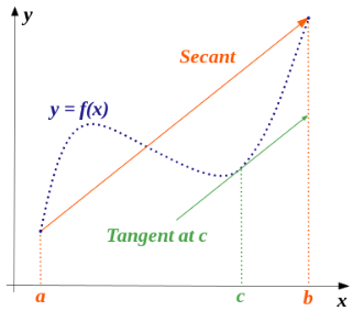
The Mean Value Theorem (MVT) for derivatives states that if the following two statements are true:
- A function is a continuous function on a closed interval [a,b], and
- If the function is differentiable on the open interval (a,b),
…then there is a number c in (a,b) such that:

The Mean Value Theorem is an extension of the Intermediate Value Theorem.
The special case of the MVT, when f(a) = f(b) is called Rolle’s Theorem.
There is also a mean value theorem for integrals.
Watch the video for an overview and a simple example, or read on below:
The Common Sense Explanation
The “mean” in mean value theorem refers to the average rate of change of the function. It’s basic idea is: given a set of values in a set range, one of those points will equal the average. This is best explained with a specific example.

Let’s say you travel from your house to work, varying your speed between 40 and 50 mph. The speedometer needle will fluctuate between 40 and 50, and let’s say you average 45 mph. As the needle moves from 40 to 50, it has to pass this point at least once. I picked 45 mph arbitrarily, but you could pick any number between 40 and 50 (i.e. the “closed interval”) and the needle would have to pass that point.
Mean Value Theorem Example Problem
Example problem: Find a value of c for f(x) = 1 + 3√(x – 1) on the interval [2,9] that satisfies the mean value theorem.
Note: The following steps will only work if your function is both continuous and differentiable.
Step 1: Find the derivative. This is where knowing your derivative rules come in handy. You can find the derivative for this particular function using the chain rule.
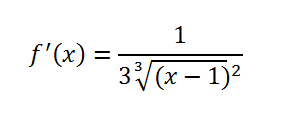
Step 2: Place your answer from Step 1 into the formula in the f′ (c) position:

Step 3: Plug in the two boundaries (from the question: 2 and 9) into the formula. “b” is the highest value on the number line, and “a” is the smallest value. Make sure you put those values in the numerator and the denominator:

Step 4: Work the right side of the equation. For f(2) and f(9), you solve by plugging each value, 2 and 9, into the formula from the question.
In other words, solve f(x) = 1 + 3√(2 – 1) and f(x) = 1 + 3√(9 – 1). I used Google’s calculator, which solves cubed roots if you type in the words (i.e. 1 + the cubed root of (2 – 1)).

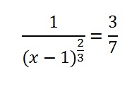
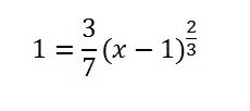
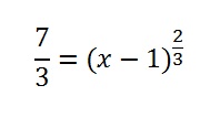
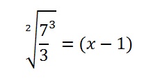
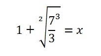
Step 5: Solve for x. Solid algebra skills will probably come into play for most questions:
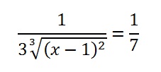
- Multiply by 3 and rewrite as 2⁄3 power.

- Multiply by (x – 1)2⁄3.

- Multiply by 7⁄3.

- Raise to 3⁄2.

- Add 1.

Note: If you have two solutions (e.g. a positive and negative value), check your interval to make sure both values are in the interval. In some cases, only one of the values will be in the interval, giving you just one solution.
Extended Mean Value Theorem
There are several “extended mean value theorems”. Most authors, when referencing the EMVT are usually referring to Cauchy’s (Extended) Mean Value Theorem although in some cases they are referring to the mean value theorem for integrals or even Taylor’s theorem.
The “Classical” Mean Value Theorem states:
For a continuous function g defined on the closed interval [a, b] and differentiable on the open interval (a, b), there is at least one number c in (a, b) for which g′(c) = (g(b) – g(a)) / (b – a).
New extensions of the MVT are being developed all of the time, for a wide variety of applications including for one-sided differentiable functions [1] and holomorphic Functions [2].
Cauchy’s Mean Value Theorem
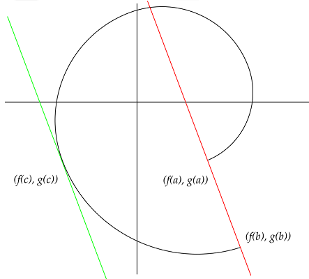
Cauchy’s (extended) mean value theorem is a generalization of the classical MVT. It is usually stated as follows: If functions f and g are continuous of the closed interval [a, b] and differentiable on the open interval (a, b), then there is at least one point c ∈ (a, b) such that:

As long as g′ (x) ≠ 0.
Geometrically, the theorem is telling us that there is a value c in the open interval (a, b) for which the tangent line to the curve at (f(c), g(c)) is parallel to the line that connects the two endpoints:
Other Extended Mean Value Theorem / Special Cases
- Rolle’s theorem: A special case of the MVT, when f(a) = f(b)
- The mean value theorem for integrals: states that somewhere under the curve of a function, there is a rectangle with an area equal to the whole area under a curve.
- Taylor’s Theorem: Although some authors refer to this as an extension of the MVT [3], it could be viewed more like an application. The MVT can be used to prove the a generalized Taylor’s theorem (with Lagrange form of the remainder term) [4] or deduce Taylor’s theorem in one variable [5].
Extreme Value Theorem
The extreme value theorem, which can be used to prove Rolle’s theorem, tells us that a continuous function contains both the maximum value and a minimum value as long as the function is:
- Real-valued,
- Defined on a closed interval, I.
Another way of saying this is that the continuous, real-valued function, f, attains its maximum value and its minimum value each at least once on the interval.
This theorem (sometimes called the maximum value theorem) is an “existence theorem”. It tells us that a max and min exist, but doesn’t tell us how to find them. It may seem too simple to be really important or significant, but it actually is the foundation for other theorems and is very significant in the groundwork of Calculus. It is used to prove Rolle’s theorem, among other things.
Examples of the Extreme Value Theorem in Action
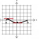
The image below shows a continuous function f(x) on a closed interval from a to b. [a,b]. The absolute maximum is shown in red and the absolute minimum is in blue.
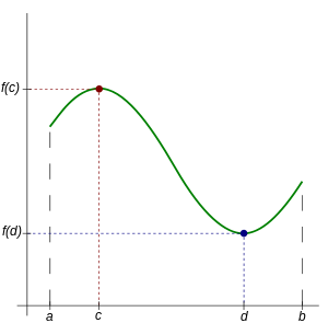
Since we know the function f(x) = x2 is continuous and real valued on the closed interval [0,1] we know that it will attain both a maximum and a minimum on this interval.
In order for the extreme value theorem to be able to work, you do need to make sure that a function satisfies the requirements:
- Real-valued,
- Continuous,
- Closed interval domain,
For example, the function f(x) = 1/x on the half open interval (0,1] doesn’t attain a maximum. That’s because the interval is not closed.
History
The extreme value theorem itself was first proved by the Bohemian mathematician and philosopher Bernard Bolzano (of Bolzano Theorem’s fame) in 1830, but his book, Function Theory, was only published a hundred years later in 1930. Another mathematician, Weierstrass, also discovered a proof of the theorem in 1860.
References
Wandzura, Jacqueline and Wandzura, Stephen. Extreme Value Theorem Demonstration. Retrieved from http://demonstrations.wolfram.com/ExtremeValueTheorem/ on August 11, 2019
Maxima and Minima. Whitman University Calculus Online. Retrieved from https://www.whitman.edu/mathematics/calculus_online/section05.01.html on October 12, 2018.
Extended Mean Value Theorem: References
[1] Slota, D. et al. (2012). Mean Value Theorems for One-Sided Differentiable Functions. PDF: http://www.math.put.poznan.pl/artykuly/FM48(2012)-WitulaR-HetmaniokE-SlotaD.pdf
[2] Cakmak, D. & Tiryaki, A. Mean Value Theorem for Holomorphic Functions. Electronic Journal of Differential Equations, Vol. 2012 (2012), No. 34, pp. 1–6.
ISSN: 1072-6691Retrieved May 6, 2021 from: https://ejde.math.txstate.edu/Volumes/2012/34/cakmak.pdf
[3] Robbin J. (2000). Taylor’s Formula (The Extended Mean Value Theorem). Retrieved May 6, 2021 from: https://people.math.wisc.edu/~robbin/221dir/taylor.pdf
[4] Yunsen, C. Mean value theorem. Retrieved May 6, 2021 from: https://www.academia.edu/23708876/Mean_value_theorem
[5] Pinkham, H. (2014). Analysis, Convexity, and Optimization. Lecture 4: Taylor’s Theorem in One Variable. Retrieved May 6, 2021 from: https://www.math.columbia.edu/~pinkham/Optimizationbook.pdf
Mean Value Theorem for Integrals
The mean value theorem for integrals states that somewhere under the curve of a function, there is a rectangle with an area equal to the whole area under a curve.
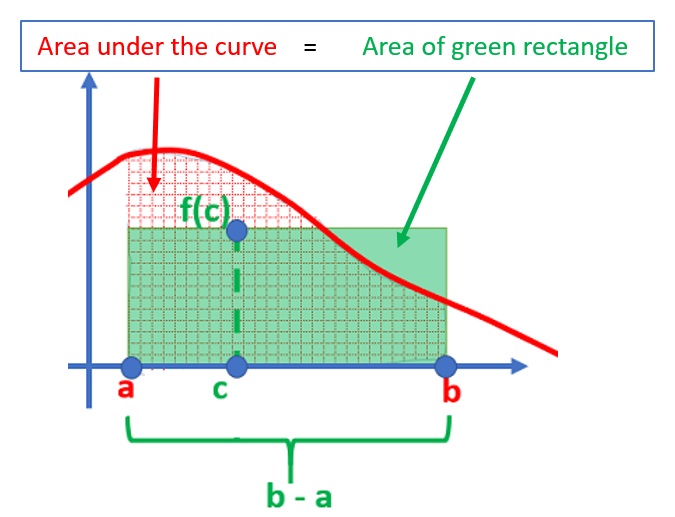
Usually, questions concerning the mean value theorem for integrals ask you to find a value for c. To answer that, you need the formal definition of the theorem.
Formal Definition of the Mean Value Theorem for Integrals
A continuous function f on a closed, bounded interval [a, b] has at least one number c in the interval (a, b) for which [1]:

In English, it’s saying that the definite integral from a to b is going to be equal, at some point, to a rectangle. The area of the rectangle is found with the equation f(c)*(a – b), which is the function value at c multiplied by the interval length.
Let’s look at an example of how you can use the formal definition to find a value for c.
Example: How to Find Point “c”
Example question: Given the function f(x) = x(1 – x), what value of c satisfies the MVT for integrals on [0, 1]?
Step 1: Find the indefinite integral

Step 2: Add the bounds of integration to your answer from Step 1. We’re looking for “c” on the interval [0, 1], so:

Step 3: Set the formula from Step 3 equal to your original function, replacing all x’s in the function with c’s.

We’re doing this because we’re looking for one specific point in the function that’s equal to the definite integral on the given bounds.
Step 4: Solve the right side of the equation (Step 3) for the integral bounds:

Step 5: Expand the left side of the equation (Step 3) and then set this equal to Step 4:
c – c2 = 1/6
Step 6: Solve for c:

For brevity, I skipped writing down all of the algebra steps of solving for c, but you can find the steps here on Symbolab.
Mean Value Theorem for Integrals: References
[1] Larson, R. & Edwards, B. (2016). Calculus. Cengage Learning.
What is Rolle’s Theorem?
Rolle’s theorem is a special case of the mean value theorem. It states that for any continuous, differentiable function with two equal values at two distinct points, the function must have a point where the first derivative is zero.
Theorem in Graphical Terms
- Take any interval on the x-axis (for example, -10 to 10). Make sure two of your function values are equal.
- Draw a line from the beginning of the interval to the end. It doesn’t matter if the line is curved, straight or a squiggle—somewhere along that line you’re going to have a horizontal tangent line where the derivative, (f′) is zero. Try it!
Rolle’s Theorem in Math Terms
The standard version of Rolle’s Theorem goes like this: Let’s say you have a function f with the following characteristics:
- It’s differentiable on the open interval (a,b),
- It is a continuous function on the closed interval [a,b],
- f(a) = f(b).
Then there is some c, with a ≤ c ≤ b such that f′(c) = 0.
This is illustrated by the diagram below, which shows a real-valued, continuous function on a closed interval. According to our theorem, the function equals itself at the two endpoints of the interval means that there is a point where the tangent line is horizontal.
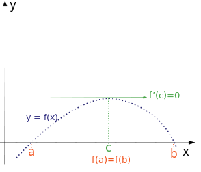
Note that Rolle’s lemma tells us that there is a point with a derivative of zero, but it doesn’t tell us where it is. It doesn’t give us a method of finding that point either. Still, this theorem is important in calculus because it is used to prove the mean-value theorem.
How to use Rolle’s Theorem
Example question: Use Rolle’s theorem for the following function:
f(x) = x2 – 5x + 4 for x-values [1, 4]
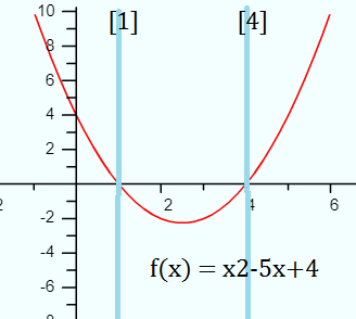
Step 1: Find out if the function is continuous. You can only use Rolle’s theorem for continuous functions.
This function f(x) = x2 – 5x + 4 is a polynomial function. Polynomials are continuous for all values of x. (How to check for continuity of a function).
Step 2: Figure out if the function is differentiable. If it isn’t differentiable, you can’t use Rolle’s theorem. the easiest way to figure out if the function is differentiable is to simply take the derivative. If you can take the derivative, then it’s differentiable.
f′(x) = 2x – 5
Step 3: Check that the derivative is continuous, using the same rules you used for Step 1.
f′(x) = 2x – 5 is a continuous function.
If the derivative function isn’t continuous, you can’t use Rolle’s theorem.
Step 4: Plug the given x-values into the given formula to check that the two points are the same height (if they aren’t, then Rolle’s does not apply).
- f(1) = 12 -5(1) + 4 = 0
- f(4) = 42 -5(4) + 4 = 0
Both points f(1) and f(4) are the same height, so Rolle’s applies.
Step 5: Set the first derivative formula (from Step 2) to zero in order to find out where the function’s slope is zero.
- 0 = 2x – 5
- 5 = 2x
- x = 2.5
The function’s slope is zero at x = 2.5.
That’s it!
History
Rolle’s theorem has a long history: we have reason to believe it was known by Indian mathematician Bhaskara II, who lived between 1114-1185. It is named after Michel Rolle, who published a proof of the polynomial case in 1691. The name was first used in 1834, by mathematician and philosopher Moritz Wilhelm Drobisch.
References
Ghosh, J. (2004). How to Learn Calculus of One Variable. New Age International.
Hosch, Wiliam L. Rolle’s. Encyclopædia Britannica
Publisher: Encyclopædia Britannica, inc. Date Published: August 05, 2011
Retrieved from https://www.britannica.com/science/Rolles-theorem
on April 04, 2019
