Riemann Sums Contents (click on a topic to go to that section):
See also: Errors in the Trapezoidal Rule and Simpson’s Rule.
Riemann Sums Definition
A Riemann sum is a way to approximate the area under a curve using a series of rectangles; These rectangles represent pieces of the curve called subintervals (sometimes called subdivisions or partitions). Different types of sums (left, right, trapezoid, midpoint, Simpson’s rule) use the rectangles in slightly different ways.
1. Left-Hand Riemann Sums
With the left-hand sum, the upper-left corner of each rectangle touches the curve.
The left-hand rule gives an underestimate of the actual area.
Back to Top
2. Right-Hand Riemann Sums
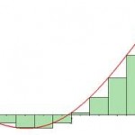
The right-hand Riemann sum approximates the area using the right endpoints of each subinterval.
With the right-hand sum, each rectangle is drawn so that the upper-right corner touches the curve.
The right-hand rule gives an overestimate of the actual area.
Back to Top
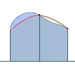
3. Trapezoid Rule
The trapezoid rule uses an average of the left- and right-hand values. While the left-hand rule, the right-hand rule and the midpoint rule use rectangles, The trapezoid rule uses trapezoids.
The trapezoids hug the curve better than left- or right- hand rule rectangles and so gives you a better estimate of the area.
4. Midpoint Rule
The midpoint rule uses the midpoint of the rectangles for the estimate. A midpoint rule is a much better estimate of the area under the curve than either a left- or right- sum. As a rule of thumb, midpoint sums are twice as good than trapezoid estimates.
Click here for Midpoint Example
5. Simpson’s Rule
Simpson’s rule uses parabolas and is an extremely accurate approximation method. It will give the exact area for any polynomial of third degree or less.
Simpson’s rule uses a combination of the midpoint rules and trapezoid rules, so if you have already calculated the midpoint (M) and trapezoid (T) areas, it’s a simple way to get a more accurate approximation.
The subscript 2n in the equation means that if you use M1 and T1, you get S2, if you use M2 and T2, you get S4.
S2n = (Mn+Mn+Tn) ⁄ 3
Example Problem (Right Hand Riemann)
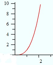
Example problem: Find the area under the curve from x = 0 to x = 2 for the function x3 using the right endpoint rule.
Step 1: Sketch the graph:
Step 2: Draw a series of rectangles under the curve, from the x-axis to the curve. We’ll use four rectangles for this example, but this number is arbitrary (you can use as few, or as many, as you like). The question asks for the right endpoint rule, so draw your rectangles using points furthest to the right. Place your pen on the endpoint (the first endpoint to the right is 0.5), draw up to the curve and then draw left to the y-axis to form a rectangle.
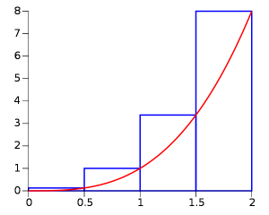
Step 3: Calculate the area of each rectangle by multiplying the height by the width.
| Interval | 0 to 0.5 | 0.5 to 1 | 1 to 1.5 | 1.5 to 2 |
| Height | 0.125 | 1 | 3.375 | 8 |
| Width | .5 | .5 | .5 | .5 |
| W * H | .0625 | .5 | 1.6875 | 4 |
Step 4: Add all of the rectangle’s areas together to find the area under the curve: .0625 + .5 + 1.6875 + 4 = 6.25
That’s it!
Tip:The number of rectangles is arbitrary—you can use as many, or as few, as you want. However, the more rectangles you use, the better the approximation will be to the actual area.
Back to Top
Example 2: Midpoint Riemann Sum
Example question: Calculate a Riemann sum for
f(x) = x2 + 2 on the interval [2,4] using n = 8 rectangles and the midpoint rule.
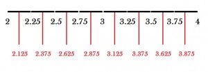
Step 1: Divide the interval into segments. For this example problem, divide the x-axis into 8 intervals.
Step 2: Find the midpoints of those segments. The midpoints for the segments (in red on the picture below) are: 2.125, 2.375, 2.625, 2.875, 3.125, 3.375, 3.625, and 3.875. These will be your inputs (x-values) for the Riemann sum.
Step 3: Plug the midpoints into the function, and then multiply by the interval length, which is 0.25:
f(2.125)0.25 + f(2.375)0.25 + f(2.625)0.25 + f(2.875)0.25 + f(3.125)0.25 + f(3.375)0.25 + f(3.625)0.25 + f(3.875)0.25
Using algebra to rewrite:
= [f(2.125) + f(2.375) + f(2.625) + f(2.875) + f(3.125) + f(3.375) + f(3.625) + f(3.875)]0.25
Plugging the function’s values into the equation:
= [6.515625 + 7.640625 + 8.890625 + 10.265625 + 11.765625 + 13.390625 + 15.140625 + 17.015625]0.25
= 90.625(0.25) = 22.65625
The midpoint came pretty close to the actual integral (22.6666).
That’s it!