- What is a Discontinuous Function?
- Graph of a Discontinuous Function
- Finding Discontinuities
- Types of Discontinuity
What is a Discontinuous Function?
A discontinuous function is a function which is not continuous at one or more points. Most functions are, perhaps surprisingly, discontinuous in one way or another [1].
Being “continuous at every point” means that at every point a:
- The function exists at that point. If you can plug an x-value into your function and it returns a value, it’s continuous at that point.
- The limit of the function as x goes to the point a exists. In other words, the function values surrounding point “a” are all approaching the same number.
- Both (1) and (2) are equal.
In notation, we can write that as:
In plain English, what that means is that the function passes through every point, and each point is close to the next: there are no drastic jumps (unlike jump discontinuities). When you’re drawing the graph, you can draw the function from left to right without taking your pencil off the paper.
A discontinuous function is one for which you must take the pencil off the paper at least once while drawing.
Graph of a Discontinuous Function
Graphically, a discontinuous function will either have a hole—one spot, or several spots, where the function is not defined—or a jump, where the value of f(x) changes (“jumps”) quickly as you go from one spot to another that is infinitesimally close.
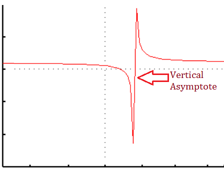
It might also have an asymptote, a line where, as the function approaches, it goes to infinity. The function never merges with this line, though it may approach infinitely close.
Finding Discontinuities
If your function can be written as rational function (i.e. a fraction), any values of x that make the denominator go to zero will be discontinuities of your function. Those are the places your function is not defined because of division by zero.
If you have a piecewise function, the point where one piece ends and another piece ends are also good places to check for discontinuity.
Otherwise, the easiest way to find discontinuities in your function is to graph it. Take note of any holes, asymptotes, or jumps. These all represent discontinuities, and just one discontinuity is enough to make your function a discontinuous function.
See also: Continuity Test.
Types of Discontinuity
Classifying types of discontinuity is more difficult than it appears, due to the fact that different authors classify them in different ways. For example:
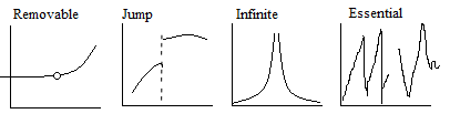
- Some authors simplify the types into two umbrella terms: removable (holes) and non-removable (jumps, infinite and essential discontinuities cannot be removed as they are too far apart or wild in their behavior).
- Essential discontinuities (that jump about wildly as the function approaches the limit) are sometimes referred to as the “non-removable discontinuity”, excluding jumps and infinite from the definition of non-removable.
- Some authors also include “mixed” discontinuities as a type of discontinuity, where the discontinuity is a combination of more than one type.
The takeaway: There isn’t “one” classification system for types of discontinuity that everyone agrees upon. Which system you use will depend upon the text you are using and the preferences of your instructor. The following list should be taken as a guide, not a set in stone classification system.
Essential Discontinuity
Essential Discontinuity
An essential discontinuity (also called second type or irremovable discontinuity) is a discontinuity that jumps wildly as it gets closer to the limit. This makes it difficult to remove the gap (hence the alternate name, “irremovable” discontinuity) and perform any calculations on the function.
An essential discontinuity is considered to be the “worst” of the types of discontinuity. That’s because the behavior around where the limits should be is abnormal, impossible to calculate, and sometimes just completely baffling. There might be many jump discontinuities within a very short distance, or you might not be able to pin down any kind of behavior at all. Graphing calculators might not be any help (because of the aberrant behavior), and you might have to resort to pen and paper to make any sense of the graph.
Subtypes
Essential discontinuities (i.e. non-removable discontinuities) can be further broken down into two types of discontinuity, based on whether the one-sided limits are bounded or unbounded (Bauldry, 2011):
- Bounded: oscillatory discontinuity. The pattern near the limit bounces up and down, never forming a pattern you can pin down.
- Unbounded: infinite discontinuity. The limits exist, but they are infinite, getting larger as you move closer to the limit.
Simple (removable) discontinuities can also be broken down into two subtypes:
- A removable discontinuity has a gap that can easily be filled in, because the limit is the same on both sides.
- A jump discontinuity at a point has limits that exist, but it’s different on both sides of the gap.
In either of these two cases the limit can be quantified and the gap can be removed; An essential discontinuity can’t be quantified. Note that jump discontinuities that happen on a curve can’t be removed, and are therefore essential (Rohde, 2012).
Essential Singularity
An essential singularity is an ill-behaved “hole” in a non-analytic complex function that can’t be removed / repaired. In other words, there’s no easy way to turn a function with an essential singularity into one that’s continuous and differentiable.
This type of singularity is similar to its real-valued counterpart: the essential discontinuity. These types of singularities / discontinuities are difficult to deal with because of their pathological behavior at a certain point.
Essential singularities are one of three types of singularity in complex analysis. The other two are poles (isolated singularities) and removable singularities, both of which are relatively well behaved. Essential singularities are classified by exclusion: if it isn’t a pole or a removable singularity, then it’s an essential one.
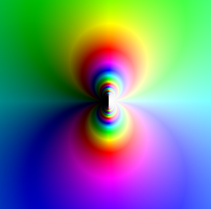
Example of a Function with an Essential Singularity
The function exp (1/z) has an essential singularity at z = 0, where the function is undefined (because of division by zero). At this point, the function does not have a limit, so it’s impossible to remove the singularity.
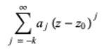
In Terms of the Laurent Series
Essential discontinuities can be identified by looking at the behavior of a Laurent series representing the neighborhood around a singularity. Specifically, a singularity is essential if the principal part of the Laurent series has infinitely many nonzero terms (Kramer, n.d.).
Infinite Discontinuity
An infinite discontinuity has one or more infinite limits—values that get larger and larger as you move closer to the gap in the function. An infinite discontinuity is a subtype of essential discontinuities, which are a broad set of badly behaved discontinuities that cannot be removed.

It’s important to note that only one side has to tend to ±infinity in order for the discontinuity to be classified as infinite. One side may reach a certain function value, or be undefined. But as long as one side is either negative infinity or positive infinity, then it’s an infinite discontinuity.
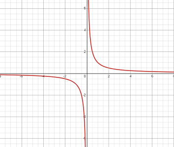
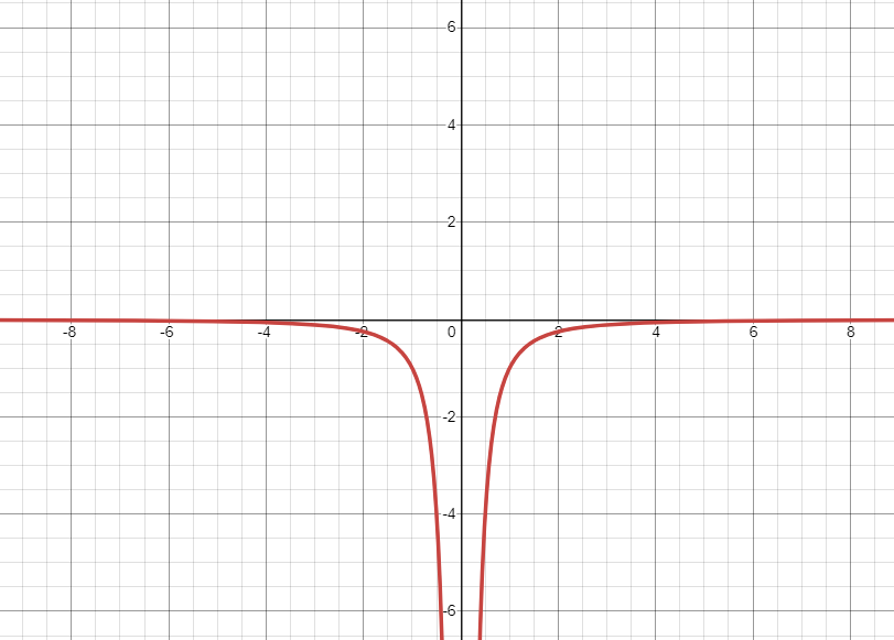
Infinity can be Positive or Negative
The function can go towards infinity in the same direction, or in different directions. For example, the function can go towards:
- Positive infinity on both sides,
- Negative infinity on both sides, or
- One side can go to negative infinity and the other towards positive infinity.
Jump Discontinuity
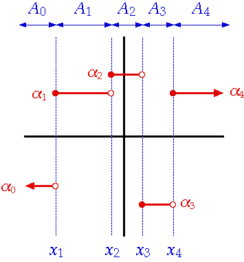
A jump discontinuity (also called a step discontinuity or discontinuity of the first kind) is a gap in a graph that jumps abruptly.
The following graph jumps at the origin (x = 0).
In order for a discontinuity to be classified as a jump, the limits must:
- exist as (finite) real numbers on both sides of the gap, and
- cannot be equal. If the limits are equal, it’s a hole, not a jump (more formally, holes are called removable discontinuities).
The difference between the two limits is the jump at that point (Sohrab, 2003). Surprisingly, the number of jumps in any particular function are countable; In other words, it’s not possible to have an infinite number of jumps, even in continuous functions (Sohrab, 2003).
When do Jumps Happen?
A jump discontinuity usually only happens in piecewise or step functions.
Piecewise functions are defined on a sequence of intervals.
Step functions are a sub-type of piecewise functions, where there’s a series of identical “staircase” steps.
Notation for Jump Discontinuities
In notation, a jump discontinuity can be defined in terms of limits on either side of the jump. Let’s say you have a function, f(t), which has a jump discontinuity at t = 10. The following notation describes the jump:
Left limit:
![]()
Right limit:
![]()
The jump itself can be defined in terms of the two limits:
f (10 +) – f (10 -).
Jump vs. Step
Although “step discontinuity” is a fairly common term, it tends to be an informal one. The usual name for this type of discontinuity is a jump discontinuity. However, when it looks like a physical step, it makes sense to call it that (rather than a jump, which would bring to mind a large gap in the horizontal axis, which isn’t always the case!). Which term you use is usually a matter of personal choice, or the choice of your instructor.
Examples of Step Discontinuity / Jump Discontinuity
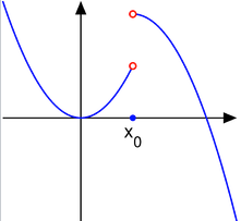
The function
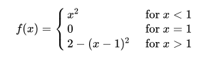
has a jump discontinuity when x = 1. There is no single limit at this point; even though the one sided limits L– and L+ both exist, because they are not equal. If you imagined walking along the curve, you would have to do some serious jumping when you got to one. This is illustrated below.
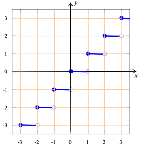
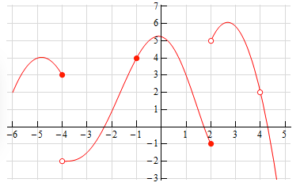
In the graph below, there is a step discontinuity at -4, because the left and right hand limits both exist and are not infinite but are different. At 2 there is another step discontinuity; the right limit is -1 and the left limit is 5. The discontinuity at 4, however, is not a step discontinuity because the left and right hand limits are equal. This is another type of discontinuity—a removable discontinuity.
What is an Oscillating Discontinuity?
An oscillating discontinuity (also called an infinitely oscillating discontinuity) jumps about wildly (i.e. oscillates) as it approaches the limit; there’s no way to “repair” the discontinuity. It’s often defined by exclusion: it isn’t a removable discontinuity, a jump discontinuity, or an infinite discontinuity. Therefore, you might see it referred to as an “other” type of discontinuity.
Bounded and Unbounded Functions
Oscillating discontinuities are bounded. In other words, their oscillations stay between certain lines. For example, the function might be bounded between a high point of y = 3 and a low point of y = -3. If the function is unbounded at one or both sides, it’s an infinite discontinuity. In other words, the function must be completely bounded at all points in order for there to be an oscillating discontinuity. In addition, the one sided limits do not exist at all.
Example
Perhaps not surprisingly, many oscillating functions have at least one oscillating discontinuity.
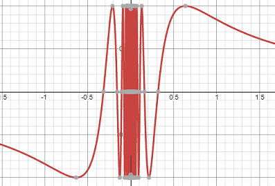
Oscillating discontinuities are a sub-type of essential, or non-repairable, discontinuities.
How to Find an Oscillating Discontinuity
The easiest way to identify this type of discontinuity is by continually zooming in on a graph: no matter how many times you zoom in, the function will continue to oscillate around the limit.
On the TI-89, graph the function in a small window (for example, a [-2,2,1]*[-2, 2, 1] window. Press the Zoom key, select the Zoom Box feature (1:ZBox) and press Enter. Mark the upper left of the box by pressing Enter, then enlarge the box using the arrow keys. Press Enter again. Repeat ad infinitum. For full instructions and images of how to do this, see: Module 8: Continuity on the TI website.
What is a Removable Discontinuity?
A removable discontinuity (also called a hole discontinuity) has a gap that can easily be filled in, because the limit is the same on both sides. You can think of it as a small hole in the x-axis.
A removable discontinuity is sometimes called a point discontinuity, because the function isn’t defined at a single (miniscule point).
Removing The Hole
The hole is called a removable discontinuity because it can be filled in, or removed, with a little redefining of the function’s values. Simply replace the function value at the hole with the value of the limit.
Example
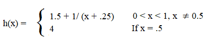
Take the following piecewise function:
Graphed, the function looks like this:
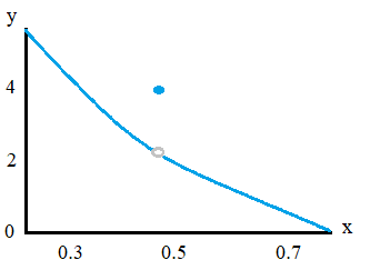
Note the small hole at x = 0.5. The function value here (i.e. the y-value) is 4, creating a problem if we want to perform further calculations on the function (like integration, for example).
On the graph, you can just pencil the hole in and remove the dot at (0.5, 4). Mathematically, if we take the y-values very close to the hole, we can fill it in that way. The piecewise function is given as h(x) = 1.5 + 1 / (x + .25) for every point except 0.5, so we can ignore that quirk and simply use the function to fill in the hole. Substituting x = 0.5 into the function, we get:
h(x) = 1.5 + 1 / (0.5 + .25) = 17/6 ≈ 2.83.
Types of Discontinuity: References
Image: Functor Salad [CC BY-SA 3.0 (http://creativecommons.org/licenses/by-sa/3.0/)]
[1] Drago et. al. A “Bouquet” of Discontinuous Functions for Beginners in Mathematical Analysis. Retrieved July 13, 2021 from: http://ceadserv1.nku.edu/longa//classes/mat420/days/highlights/PathologicalFunctions.pdf
[2] Section 1.4. Continuity. Retrieved July 13, 2021 from: https://www.math.uh.edu/~beatrice/143114.pdf
Bauldry, W. (2011). Introduction to Real Analysis: An Educational Approach. John Wiley & Sons.
Bogley, W. (1996). Removable Discontinuities. Retrieved October 28, 2019 from: https://oregonstate.edu/instruct/mth251/cq/Stage4/Lesson/removable.html
Grigoriu, M. Stochastic Calculus: Applications in Science and Engineering.
Infinite Discontinuity. Retrieved October 29, 2019 from: http://www-math.mit.edu/~djk/18_01/chapter02/example03.html
Infinite Discontinuities. Retrieved October 28, 2019 from: https://ocw.mit.edu/courses/mathematics/18-01sc-single-variable-calculus-fall-2010/1.-differentiation/part-a-definition-and-basic-rules/session-5-discontinuity/MIT18_01SCF10_Ses5c.pdf
Knopp, K. “Essential and Non-Essential Singularities or Poles.” §31 in Theory of Functions Parts I and II, Two Volumes Bound as One, Part I. New York: Dover, pp. 123-126, 1996.
Kramer, P. L.S. Examples. Retrieved August 22, 2020 from: http://eaton.math.rpi.edu/faculty/Kramer/CA13/canotes111113.pdf
Krantz, S. G. “Removable Singularities, Poles, and Essential Singularities.” §4.1.4 in Handbook of Complex Variables. Boston, MA: Birkhäuser, p. 42, 1999.
Rohde,U. et al. (2012). Introduction to Differential Calculus: Systematic Studies with Engineering Applications for Beginners. John Wiley and Sons.
Sohrab, H. (2003). Basic Real Analysis. Springer Science and Business Media.
Thomson, B. et al., (2008). Elementary Real Analysis, Volume 1. ClassicalRealAnalysis.com.
Wineman, A. & Rajagopal, K. (2000). Mechanical Response of Polymers: An Introduction. Cambridge University Press.