Serial Correlation / Autocorrelation: Definition, Tests

Statistics Definitions > Serial Correlation / Autocorrelation

What is Serial Correlation / Autocorrelation?

Serial correlation (also called Autocorrelation) is where error terms in a time series transfer from one period to another. In other words, the error for one time period a is correlated with the error for a subsequent time period b. For example, an underestimate for one quarter’s profits can result in an underestimate of profits for subsequent quarters. This can result in a myriad of problems, including:

• Inefficient Ordinary Least Squares Estimates and any forecast based on those estimates. An efficient estimator gives you the most information about a sample; inefficient estimators can perform well, but require much larger sample sizes to do so.
• Exaggerated goodness of fit (for a time series with positive serial correlation and an independent variable that grows over time).
• Standard errors that are too small (for a time series with positive serial correlation and an independent variable that grows over time).
• T-statistics that are too large.
• False positives for significant regression coefficients. In other words, a regression coefficient appears to be statistically significant when it is not.

Types of Autocorrelation

The most common form of autocorrelation is first-order serial correlation, which can either be positive or negative.

• Positive serial correlation is where a positive error in one period carries over into a positive error for the following period.
• Negative serial correlation is where a negative error in one period carries over into a negative error for the following period.

Second-order serial correlation is where an error affects data two time periods later. This can happen when your data has seasonality. Orders higher than second-order do happen, but they are rare.

Testing for Autocorrelation

You can test for autocorrelation with:

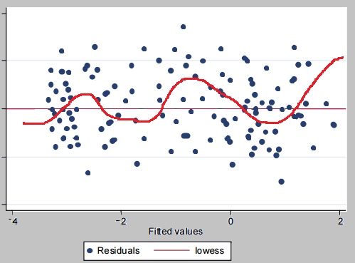
• A plot of residuals. Plot e_t against t and look for clusters of successive residuals on one side of the zero line. You can also try adding a Lowess line, as in the image below.
• A Durbin-Watson test.
• A Lagrange Multiplier Test.
• Ljung Box Test.
• A correlogram. A pattern in the results is an indication for autocorrelation. Any values above zero should be looked at with suspicion.
• The Moran’s I statistic, which is similar to a correlation coefficient.