Transformations in Statistics: Log, Reciprocal, Vector, Linear…

Definitions > Transformations in Statistics

Contents (Click to skip to that section):

1. What are Transformations in Statistics?
2. Common Transformation Types (for data)
   1. Transformations in Geometry
   2. Log Transformation
   3. Vector Transformation
   4. Linear Transformation
   5. Reciprocal Transformation
3. How to Graph Transformations
4. Other Transformations in Matrices, Regression & Hypothesis Testing
5. Why Do We Need Transformations in Statistics?
6. Implications of Transformations in Statistics

See also: Affine Transformation

What are Transformations in Statistics?

In layman’s terms, you can think of a transformation as just moving an object or set of points from one location to another. You literally “transform” your data into something slightly different.

For example, you can transform the sequence {4, 5, 6} by subtracting 1 from each term, so the set becomes {3, 4, 5}.

The many reasons why you might want to transform your data include: reducing skew, normalizing your data or simply making the data easier to understand. For example, the familiar Richter scale is actually a logarithmic transformation: an earthquake of magnitude 4 or 6 is easier to understand than a magnitude of 10,000 or 1,000,000.

More formally, transformations over a domain D are functions that map a set of elements of D (call them X) to another set of elements of D (call them Y). The relationships between the elements of the initial set are typically preserved by the transformation, but not necessarily preserved unchanged. The image below shows a piece of coding that, with four transformations (mappings) converts a simple rectangular repeated pattern into a rhombic pattern [1].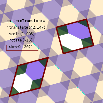

Types of transformations in statistics

The three main methods of data transformations in statistics are [2]:

• Monotonic Transformations safeguard the order of data points. In other words, if a data point is greater than another data point before the transformation, it will remain larger afterward. These transformations are often applied to make data more normally distributed. Monotonic transformations include logarithmic, exponential and reciprocal transformations.
• Relativizations (standardization) adjust the scale of the data without altering the order of data points. This means a data point that’s twice as large as another before the transformation will be twice as large afterward. This method is often used to simplify data interpretation. Standardization transformations include square root, cube root and logit transformation.
• Probabilistic Transformation (smoothing) modify the shape of the distribution. For example, if a dataset is normally distributed before the transformation, it may not maintain this distribution afterward. These transformations are commonly used to make data more suitable for statistical analysis. Probabilistic transformations include Beta, Gamma, and Poisson transformations.

The most useful transformations in statistics and introductory data analysis are the cube root, logarithm, square root, and square [3]:

• Cube Root Transformations: x → x^(⅓) can reduce right skewness for zero and positive values. The cube root transformation significantly alters the shape of the distribution. A unique aspect of this transformation is that the cube root of a negative number has the same absolute value as the cube root of the equivalent positive number, but with a negative sign. This property holds for any root whose power is the reciprocal of an odd positive integer (powers 1/3, 1/5, 1/7, etc.). However, this property is sensitive; even a slight change from 1/3, and the result can no longer be defined as a product of precisely three terms.
• Log Transformation, x to log(x), takes the natural logarithm of variables in a data set and is commonly used to reduce right skewness. This strong transformation has a big effect on the shape of the distribution. It can’t be applied to zero or negative values.
• Taking the square: x → x² can reduce left skewness. It has a medium effect on the shape of data and can help reduce left skewness. It’s often used to fit a response by a quadratic function y = a + b x + c x². Quadratics have a turning point, either a maximum or minimum, which may be beyond the limits of observations in a fitted function. Quadratics are typically used because they can mimic a relationship within the data region, but they might behave poorly outside that region due to large values for extreme x values. Squaring is usually appropriate only for zero or positive variables, as (-x)² and x² are identical.

Other types of transformations in statistics include:

• A Box Muller Transform turns uniformly distributed data into normally distributed data.
• Differencing: although most transformations preserve elements in the initial set, differencing results in one less data point than the original data. For example, given a series Z_t differencing can create a new series Y_i = Z_i – Z_i – 1.
• Fitting a curve: In modeling, you may want to model residuals from a fitted curve. Curve fitting algorithms that can help with this task include: Gauss-Newton, gradient descent, and the Levenberg–Marquardt algorithm.
• The reciprocal transformation x → 1/x results in a drastic change on a distribution’s shape, reversing the order of values with the same sign; The negative reciprocal, x to -1/x, also has a large effect but preserves the order of variables. This can be a useful transformation for a set of positive variables where a reverse order makes more sense. For example, instead of number of patients per doctor, you can transform to number of doctors per patient [3].
• Square root transformations take the square root of variables, e.g., x → x^(½) = sqrt(x). While square root transforms have a moderate effect on the shape of the distribution, it is considered to be weaker than logarithmic or cube root transformations. It is used for data with non-constant variance.

The relationships between the elements of the initial set are usually preserved by the transformation, but not necessarily preserved unchanged.

Transformations in calculus and geometry

In calculus and geometry, types of transformations include translations (shifts, scales, and reflections) rotation, and shear mapping. But more generally, a transformation can mean any kind of mathematical function. In general, you can transform a function in seven basic ways. For a function y = f(x):

• y = f(x – c): Horizontal shift c units right
• y = f(x + c): Horizontal shift c units left
• y = f(x) – c: Vertical shift c units down
• y = f(x) + c: Vertical shift c units up
• y = -f(x): Reflection over the x-axis
• y = f(-x): Reflection over the y-axis
• y = -f(-x): Reflection about the origin.

1. Shift: moves every point by the same distance in the same direction.
2. Reflection: a folding or flipping over a certain line (e.g., the y-axis).
3. Glide reflections: a combination of a reflection and a shift.
4. Rotation: turns a figure about a fixed point (a center of rotation).
5. Scaling: Enlarges, or shrinks, an object by the same scale factor.
6. Shear mapping: all points along one line stay fixed, while other points are shifted parallel to the line by a distance proportional to their perpendicular distance from the line.

 

Using transformations to graph functions

Sometimes we can use the concept of transformations to graph complicated functions when we know how to graph the simpler ones.

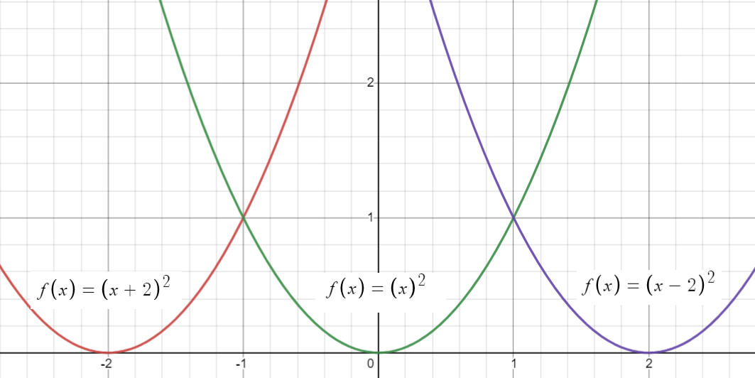
For example, if you know the graph of f(x), the graph of f(x) + c will be the same function, just shifted up by c units. f(x) – c will be the same thing, too, just shifted down by c units. The graph of f(x + c) s the graph of f(x), shifted left by c units, and the graph of f(x – c) is the graph of f(x) shifted right by c units.

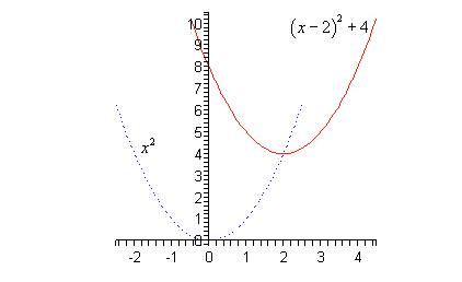
For a few step by step examples of vertical (up/down) shifts, see: Vertical Shift of a Function As an example, take the graph of

f(x) = (x – 2)² + 4.

We might not know what that looks like, but we do know what h(x) = x² looks like—a simple upward facing parabola. Imagine sketching that, then shift it to the right by 2 and up by 4. Then you have the sketch of f(x).

Vector transformation

A vector transformation is a specific type of mapping where you associate vectors from one vector space with vectors in another space.

The concept of a vector space is fundamental to understanding vector transformations. A vector space is a collection of vectors which can be added and multiplied by scalars. Vectors have both magnitude and direction (e.g. 10 mph East). A vector space has two requirements. Without leaving the vector space,

• Any two vectors can be added.
• Any two vectors can be scaled (multiplied).

Vector Spaces are often defined as Rⁿ vector spaces, which are spaces of dimension n where adding or scaling any vector is possible. R stands for “Real” and these spaces include every vector of the same dimension as the space. For example, the R² vector spaces includes all possible 2-D vectors.

• The vectors (4, 2), (19, 0), and (121, 25) are all 2-D vectors (ones that can be represented on an x-y axis).
• The vector space R³ represents three dimensions,
• R⁴ represents four dimensions and so on.
• It’s practically impossible to deal with Rⁿ vector spaces, because they contain every possible vector of n dimensions, up to infinity. Instead, we use subspaces, which are smaller vector spaces within a Rⁿ vector space. 

Back to Top

Vector transformations can be thought of as a type of function. For example, if you map the members of a vector space Rⁿ to unique members of another vector space Rp, that’s a function. It’s written in function notation as: f: Rⁿ → R^p

Let’s say you had a vector transformation that mapped vectors in an R³ vector space to vectors in an R² space. The general way to write the notation is: f: R³ → R² A specific example: f(x₁, x₂, x₃) = (x₁ + 3x₂, 4x₃) Note that f(x₁, x₂, x₃) has three vectors and so belongs in ℝ³ and (x₁ + 3x, 4x₃) has two vectors and so belongs in ℝ². This example could also be written as: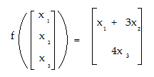
Working out the vector transformation is equivalent to working out a function and involves some basic math. For example, let’s say you had the function f: x→ x² and you wanted to transform (map) the number 2. You would insert it into the right hand part of the equation to get 2² = 4. Vector transformation works the same way.

For example, performing a vector transformation from f(2, 3, 4) to (X₁ + 3x₂, 4x₃) we get:

• X₁ = 2
• X₂ = 3
• X₃ = 4,

so: (2 + 3(3), 4(4)) = (2 + 9, 16) = (11, 16)

Back to Top

Linear Transformation

Linear transformation is a special case of a vector transformation.   Definition: Let V And W be two vector spaces. The function T:V→W is a linear transformation if the following two properties are true for all u, v, ε, V and scalars C:

1. Addition is preserved by T: T(u + v) = T(u) = T(v). In other words, if you add up two vectors u and v it’s the same as taking the transformation of each vector and then adding them.
2. Scalar multiplication is preserved by t: T(cu) = cT(u). In other words, if you multiply a vector u by a scalar C, this is the same as the transformation of u multiplied by scalar c.

Applying rules 1 and 2 above will tell you if your transformation is a linear transformation.  Part One, Is Addition Preserved? Works through rule 1 and Part Two, Is Scalar Multiplication Preserved? works through rule 2. Remember: Both rules need to be true for linear transformations.

Example Question: Is the following transformation a linear transformation? T(x,y)→ (x – y, x + y, 9x)

1. Give the vectors u and v (from rule 1) some components. I’m going to use a and b here, but the choice is arbitrary:
   • u = (a₁, a₂)
   • v = (b₁, b₂)
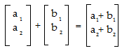
2. Find an expression for the addition part of the left side of the Rule 1 equation (we’re going to do the transformation in the next step): (u + v) = (a₁, a₂) + (b₁, b₂) Adding these two vectors together, we get: ((a₁ + b₁), (a₂ + b₂)) In matrix form, the addition is:
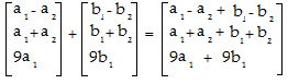
3. Apply the transformation. We’re given the rule T(x,y)→ (x – y, x + y, 9x), so transforming our additive vector from Step 2, we get:
   • T ((a₁ + b₁), (a₂+ b₂)) =
   • ((a₁ + b₁) – (a₂ + b₂),
   • (a₁ + b₁) + (a₂ + b₂),
   • 9(a₁ + b₁)).

   Simplifying/Distributing using algebra: (a₁ + b₁ – a₂ – b₂, a₁ + b₁ + a₂ + b₂, 9a₁ + 9b₁). Set this aside for a moment: we’re going to compare this result to the result from the right hand side of the equation in a later step.

4. Find an expression for the right side of the Rule 1 equation, T(u) + T(v). Using the same a/b variables we used in Steps 1 to 3, we get: T((a₁,a₂) + T(b₁,b₂))
5. Transform the vector u, (a₁,a₂). We’re given the rule T(x,y)→ (x – y, x + y, 9x), so transforming vector u, we get:
   • (a₁ – a₂,
   • a₁ + a₂,
   • 9a₁)
6. Transform the vector v. We’re given the rule T(x,y)→ (x – y, x + y,9x), so transforming vector v, (a₁,a₂), we get:
   • (b₁ – b₂,
   • b₁ + b₂,
   • 9b₁)
7. Add the two vectors from Steps 5 and 6: (a₁ – a₂, a₁ + a₂, 9a₁) + (b₁ – b₂, b₁ + b₂, 9b₁) = ((a₁ – a₂ + b₁ – b₂, a₁ + a₂ + b₁ – b₂, 9a₁ + 9b₁)

   

8. Compare Step 3 to Step 7. They are the same, so condition 1 (the additive condition) is satisfied.

Next, we want to know if scalar multiplication is preserved. In other words, in this part we want to know if

T(cu)=cT(u) is true for T(x,y)→ (x-y,x+y,9x).

We’re going to use the same vector from Part 1, which is u = (a₁, a₂).

1. Work the left side of the equation, T(cu). First, multiply the vector by a scalar, c. c * (a₁, a₂) = (c(a₁), c(a₂))
2. Transform Step 1, using the rule T(x,y)→ (x-y,x+y,9x): (ca₁ – ca₂, ca₁ + ca₂, 9ca₁) Put this aside for a moment. We’ll be comparing it to the right side in a later step.
3. Transform the vector u using the rule T(x,y)→ (x-y,x+y,9x). We’re working the right side of the rule 2 equation here: (T(a₁, a₂)= a₁ – a₂ a₁ + a₂ 9a₁)
4. Multiply Step 3 by the scalar, c. (c(a₁ – a₂) c(a₁ + a₂) c(9a₁)) Distributing c using algebra, we get: (ca₁ – ca₂, ca₁ + ca₂, 9ca₁)
5.  Compare Steps 2 and 4. they are the same, so the second rule is true. This function is a linear transformation.

Back to Top

An isometry is a linear transformation that preserves distance and length. The image below shows a linear transformation f that sends A to B and X to Y, while preserving the distance between the points A and B (X and Y) and the length of the line AB (XY). If A and B were 5 cm away originally, the distance between f(A) = X and f(B) = Y, must also be 5 cm.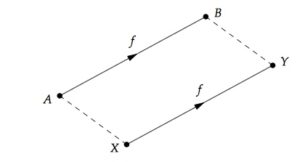
An isometry is also sometimes called a congruence transformation.

Since we call any property that is preserved under a transformation invariant under that transformation, we can say that length and distance are invariant under a congruence transformation. Rotation, shift, reflection, glides, and the identity map are all isometries. If two figures are related by a congruence transformation (can be transformed into each other by means of an isometry), they are called congruent.

The formal definition for an isometry is: If we have X and Y, two metric spaces with metrics d_X and dY, then the map f:X → Y is an isometry if, for every and any a, b in X.

d_Y(f(a)f(b)) = d_X(a,b).

In the Euclidean plane, any isometry that maps each of three non-collinear points (points that do not all lie on one line) to each other is the identity transformation (the transformation that sends every point to itself). If an isometry in the plane has more than one fixed point, it is either a reflection (over an axis which crosses that point) or the identity transformation.

The image below shows one such reflection; you can see that distances are preserved and the points in the reflection plane—for example, C—remain unchanged under the transformation. 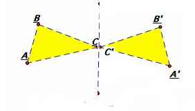Any isometry on the Euclidean plane can be uniquely determined by two sets of three non-collinear points; points that determine congruent triangles.

Log Transformation of a skewed distribution.

Log transformation means taking a data set and taking the natural logarithm of variables. Sometimes your data may not quite fit the model you are looking for, and a log transformation can help to fit a very skewed distribution into a more normal model. As a result, you can more easily see patterns in your data. Log transformation does not “normalize” your data; it’s purpose is to reduce skew.

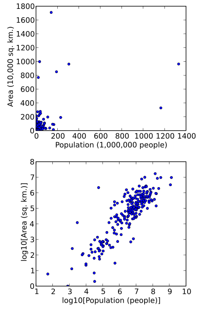
In the image above [4], it’s practically impossible to see any pattern in the above image. However, in the second image, the data has had a log transformation. Consequently, the pattern becomes apparent.

If you are running a parametric statistical test on your data (for example, an ANOVA), using data that’s highly skewed to the right or left can lead to misleading test results. Therefore, if you want to perform a test on this kind of data, run a log transformation and then run the test on the transformed numbers.

Many possible transformations exist. However, you should only use a log transformation if:

• Your data is highly skewed to the right (i.e. in the positive direction).
• The residual’s standard deviation is proportional to your fitted values
• The data’s relationship is close to an exponential model.
• You think the residuals reflect multiplicative errors that have accumulated during each step of the computation.

In SPSS: IBM’s instructions can be found here.

Reciprocal transformation

The reciprocal transformation is defined as the transformation of x to 1/x. The transformation has a dramatic effect on the shape of the distribution, reversing the order of values with the same sign. The transformation can only be used for non-zero values. A negative reciprocal transformation is almost identical, except that x maps to -1/x and preserves the order of variables.

How to graph transformations

Once you’ve committed graphs of standard functions to memory, your ability to graph transformations is simplified.

The eight basic function types are:

• Sine function,
• Cosine function,
• Rational function,
• Absolute value function,
• Square root function,
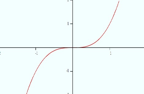
• Cube (polynomial) function,
• Square (quadratic) function,
• Linear function.

Each has their own domain, range, and shape. When you transform one of these graphs, you shift it up, down, to the left, or to the right.

Being able to visualize a transformation in your head and sketch it on paper is a valuable tool. Why? Sometimes the only way to solve a problem is to visualize the transformation in your head. While graphing calculators can be a valuable tool in developing your mathematical knowledge, eventually the calculator will only be able to help you so much.

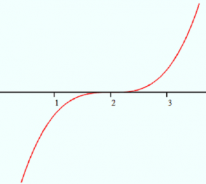
Example Problem 1: Sketch the graph of x³ shifted two units to the right and then write the equation for that graph.

1. Visualize the graph of x³, which is a cube (polynomial).
2. Visualize the transformation. All you’re doing is shifting the graph two units to the right. Here’s what the transformed graph looks like:
3. Write the equation. For any function, f(x), the graph of f(x + c) is the graph shifted to the left and the graph of f(x – c) is the graph shifted to the right. The question asks for two units (i.e. 2) to the right, so the final equation is f(x) = (x – 2)³.

Caution: the graph of x² – 2 moves the graph down two units, not right!

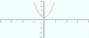
Example problem 2: Sketch the graph of x² + 2.

1. Visualize the graph of x².
2. Sketch the graph. For any function, f(x), a graph f(x) + c is the graph shifted up the y-axis and a graph f(x) – c is a graph shifted down the y-axis. Therefore, x² + 2 is the graph of x² shifted two units up the y-axis.

That’s it!

Tip: You can also flip graphs on the x-axis by adding a negative coefficient. For example, while x² is a parabola above the x-axis, -x² is a mirror image over the x-axis.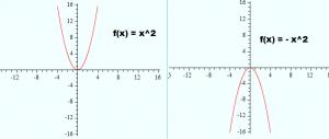

Other transformations

• A Box Cox transformation is used when you need to meet the assumption of normality for a statistical test or procedure. It transform non-normal dependent variables into a bell shape.
• Another way to normalize data is to use the Tukey ladder of powers (sometimes called the Bulging Rule), which can change the shape of a skewed distribution so that it becomes normal or nearly-normal.
• A third, related procedure, is a Fisher Z-Transformation. The Fisher Z transforms the sampling distribution of Pearson’s r (i.e. the correlation coefficient) so that it becomes normally distributed.
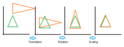
• Generalized Procrustes analysis, which compares two shapes in Factor Analysis, uses geometric transformations (i.e. rescaling, reflection, rotation, or shift) of matrices to compare the sets of data.
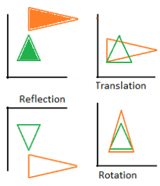
• The following image shows a series of transformations onto a green target triangle.

 

Why do we need transformations in statistics? 

Altering data can help meet specific statistical assumptions in regression and hypothesis testing, such as normality, homogeneity, and linearity. Data transformation can also help to balance values from diverse set of data to make them comparable and assist in generating more informative graphs and charts.

A couple of other examples of how transformations can be applied in statistics:

• To normalize data: If a dataset isn’t normally distributed, using statistical tests can be challenging and may give misleading results. Transformations can adjust the scale of the data, making it more normally distributed. This allows the application of statistical tests on the data, leading to more precise outcomes. For example, the t-test is used to compare the means of two groups. However, it’s only accurate if the data is normally distributed. If the data isn’t normally distributed, transformations can adjust the scale of the data, making it more normally distributed. This enhances the accuracy of the t-test.
• To simplify data interpretation: If a dataset covers a wide range of values, finding trends in the data can be difficult. Transformations can adjust the scale of the data, making trends more noticeable. This simplifies data interpretation and conclusion drawing. For example, the Richter scale is a logarithmic transformation: a mag 4 earthquake is easier to understand than a mag 10,000.

Implications of transformations in statistics

Data transformation can be beneficial in obtaining new perspectives and reducing noise in your data. However, there are a few pitfalls to watch out for, including:

• Transformations can alter the meaning of the data. For example , if you take the logarithm of each value in a dataset, you’re stating that the values are proportional to each other, which means you can’t compare the absolute values of data points post-transformation.
• Choosing the wrong transformation for the dataset. Not all transformations are suitable for all datasets. For example, if you have a normally distributed dataset, a transformation intended to make it more normally distributed wouldn’t be necessary.

Using data transformation techniques demands a thorough understanding of the effects, implications, and conclusions drawn from the transformed data. It should only be conducted only when necessary and when the goal of the transformation is clear. Your main criterion for choosing a transformation should be simply: what works with the data? [3].

Horizontal shift of a function

A horizontal shift adds or subtracts a constant to or from every x-value, leaving the y-coordinate unchanged. The basic rules for shifting a function along a horizontal (x) are:

Compared to a base graph of f(x),

1. y = f(x + h) shifts h units to the left,
2. y = f(x – h) shifts h units to the right,

Where h > 0.

Look carefully at what the positive or negative added value h is doing: it’s the opposite of what you might expect. Positive values of h shift in the negative direction along the number line and negative h values shift the positive direction.

Example: A horizontal shift of the function f(x) = x² of 2 units (i.e. h = 2) results in:

• f(x) = x² + 3 (3 units to the left),
• f(x) = x² + 3 (3 units to the right)

The following graph shows the base function f(x) = x² and the two “new” graphs created when we added 2 or subtracted 2.

 

Example question #1: How are the graphs of y = √(x) and y = √(x + 1) related?

Solution:

1. Compare the right sides of both equations and note any differences:
   • √(x)
   • √(x + 1)

   The difference between the equations is a “+ 1”.

2. Choose a rule based on whether Step 1 was positive or negative: Step 1 for this example was positive (+ 1), so that’s rule 1: y = f(x + h) shifts h units to the left
3. Place your base function (from the question) into the rule, in place of “x”: y = f(√(x) + h) shifts h units to the left
4. Place “h” — the difference you found in Step 1 — into the rule from Step 3: y = f(√(x) + 2) shifts 2 units to the left

That’s it!

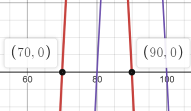
Example question #2: The following graph shows how the average cost of a new car tire compares from Jacksonville, Florida (red) to Miami, Florida (Blue). Write a formula for the transformation of g (blue graph) to f (red graph).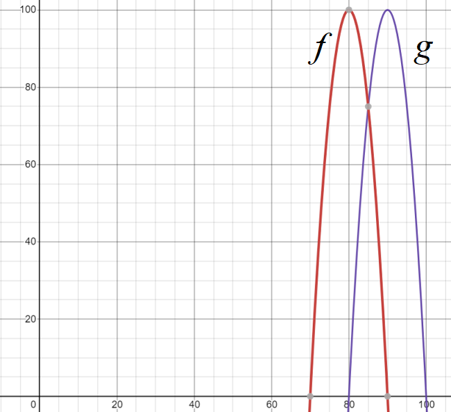

Solution: The graph g shifts 10 units to the right of f, so: g(x) = f(x – 20) . If you’re not sure about how I arrived at this formula, the following few steps break it down into simple parts:

1. Decide which direction the graph is traveling (left, or right?). The question asks is for a formula for the transformation of g (blue graph) as a transformation of f (red graph). In other words, what direction do we need to travel to turn f into g? A look at the graph shows that moves to the right.
2. Take your answer from Step 1 and then refer to the rules to tell you whether it’s a positive or negative shift. Rule 2 states: y = f(x – h) shifts h units to the right. That means moving to the right must mean we have a “-” shift. Put this value aside for a moment.
3. Locate two x-values on the horizontal axis: one for each graph:
   • g (blue graph) = 70
   • f (red graph) = 90.

   

4. Subtract the lowest number in Step 3 from the highest: 90 – 70 = 20.
5. Step 5: Combine your answers from Steps 2 and 4: – 20.
6. Step 6: Place your answer from Step 5 into the rule you chose in Step 2, replacing the “h” with your value (- 20 in this example): g(x) = f(x – 20) Don’t forget to rename the formula with the one given in the question!

References

Graph created with Desmos.com.

1. Arthur Baelde, CC BY-SA 3.0 , via Wikimedia Commons
2. McCune, B. et al. (2002)  Analysis of Ecological Communities.
3. Transformations: an introduction. Retrieved July 2, 2023 from: http://fmwww.bc.edu/repec/bocode/t/transint.html#:~:text=In%20data%20analysis%20transformation%20is,of%20a%20distribution%20or%20relationship.
4. Population vs area by Skbkekas. CC BY-SA 3.0 , via Wikimedia Commons