Intermediate Value Theorem: Definition, Examples

What is the Intermediate Value Theorem?

The basic idea behind the intermediate value theorem (IVT) is this: suppose you have a line segment (between points a and b, inclusive) of a continuous function, and that function crosses a horizontal line. Given these facts, then the intersection of the two lines—point c—must exist. The theorem is used for two main purposes:

To prove that point “c” exists,
To prove the existence of roots (sometimes called zeros of a function).

This may seem like an exercise without purpose, but the theorem has many real world applications.

A More Formal Definition

The textbook definition of the intermediate value theorem states that:

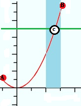
If f is continuous over [a,b], and y₀ is a real number between f(a) and f(b), then there is a number, c, in the interval [a,b] such that f(c) = y₀.

In other words, if you have a continuous function and have a particular “y” value, there must be an “x” value to match it. The theorem is also stated—a little bit more simply—as that a continuous function takes on all values between f(a) and f(b); there are no gaps or missing values.

With intermediate value theorems, you aren’t looking for a certain solution (a number), you are just proving that a number exists (or doesn’t exist). You do this by:

Checking for continuity.
Evaluating the function at some point.

Example

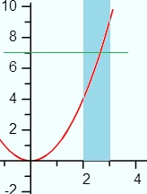
Example #1: For the function f(x) = x², show that there is a number “m” between 2 and 3 such that f(m) = 7.

Step 1: Draw a graph to help you visualize the problem.

example for the intermediate value theorem — y = 7 (green line) lies somewhere in between x= 2 and 3 (blue shaded area).

This is an optional step, but it’s good to wrap your head around exactly what you are looking for.

Step 2: Check for continuity. If the function isn’t continuous, you can’t use the intermediate value theorem. This function is a polynomial function, so we can use the theorem: all polynomials are continuous.

Step 3: Evaluate the function at the lower and upper values given. For this example, you’re given x = 2 and x = 3, so:

f(2) = 4
f(3) = 9

7 is between 4 and 9, so there must be some number m between 2 and 3 such that f(c) = 7.

That’s it!

Using the Intermediate Value Theorem to Prove Roots Exist

A second application of the intermediate value theorem is to prove that a root exists.

Example problem #2: Show that the function f(x) = ln(x) – 1 has a solution between 2 and 3.

Step 1: Solve the function for the lower and upper values given:

ln(2) – 1 = -0.31
ln(3) – 1 = 0.1

You have both a negative y value and a positive y value. Therefore, the graph crosses the x axis at some point. A quick look at the graph and you can see this is true:
ivt 2

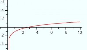
Step 2: Check that the graph is continuous. The function ln(x) is defined for all values of x > 0, so it is continuous on the interval [2,3].

That’s it!

Real World Applications of the IVT

A simple real world example of how the theory works: You measure the weight of your new puppy and she is 15 lbs. Ten days later she weights 18 lbs. That gives you two points on your closed interval:

f(a) = f(0) = 15 lbs
f(b) = f(10) = 18 lbs

Let’s say you wanted to pinpoint the moment when your puppy weighed c = 16.5 lbs. The IVT tells you that this point c must exist. It might take you a while to pinpoint that exact time, but you know your time isn’t going to be wasted. This simple example can be extended to any problem in science that involves pinpointing a specific time, weight, or other metric. For example, carbon dating an object typically takes several days to process, so it’s nice to know from the outset that a solution is possible. Invoking the IVT before you start any complicated technical process saves wasting time and resources on hunting down solutions that may or may not exist.

Some more real life examples:

At any point in time, there are two points diametrically opposite each other on the Earth’s surface that have exactly the same temperature (Devlin, 2007).
Climatologists use the IVT to make predictions about how rising carbon dioxide levels will affect our planet (CK12).
Any table that is wobbly because one leg isn’t touching the ground can be stabilized by rotating it (thus, saving napkins, and therefore, trees) (Devlin, 2007).

Darboux’s Theorem

Darboux’s Theorem (also called Darboux Continuity or Darboux Property) tells us that any derivative has the Intermediate Value Theorem property, even discontinuous ones. The IVT says that if a continuous function takes on a negative value and then switches to a positive value, it must take on a value of “0” somewhere in between.

Up until French mathematician Jean Gaston Darboux developed the proof of his theorem in 1975, it was widely believed that the IVT implied continuity. Darboux showed this wasn’t the case, demonstrating several differentiable functions with discontinuous derivatives [1].

Darboux made several contributions to the theory of singularities in differential equations. The similarly-named “Darboux theorem” concerns neighborhoods of points in manifolds [2].

Formal Definition of Darboux’s Theorem

Darboux’s Theorem is formally stated as [3]:
Suppose a function is differentiable on a closed interval [a, b] so that:

- f′(a) = y₁

and

f′(b) = y₂

If d lies between y₁ and y₂, then there is a point c in the interval [a, b] with f′(c) = d.

Darboux’s Theorem Example

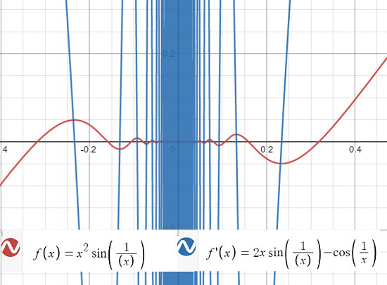
The above graph shows the function f(x) = x² sin(1/x) and its discontinuous (at zero) derivative f′(x) = 2x sin(1/x) – cos(1/x). The problem with the derivative is that the second part, cos(1/x), isn’t defined at zero. But we can assign a value by tweaking the function’s definition:

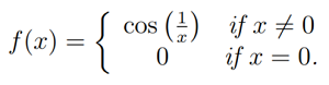
This perfectly valid definition means that the derivative now has the IVT property for certain intervals [4]. For example [0.5, 2]. But it isn’t continuous, and behaves pathologically as it nears zero.

Many different proofs can be found in the literature. Several proofs of the theorem can be found in Dr. Mukta Bhandar’s paper Another Proof of Darboux’s Theorem[5] available here.

Darboux Property

The Darboux property is another name for Darboux’s theorem. However, some authors may use a slightly different definitions, which means that the two terms may in some cases also differ. For example, Beni Bogoşel states [6] that a function has the Darboux property if, for any interval I ⊂ ℝ, f(I) is also an interval; Bogoşel clarified in a comment that he was using a seldom-used form of the intermediate value property where the entire image is an interval. Continuity implies the Darboux property and the Darboux property implies the intermediate value property.

References

[1] Olsen, L. A New Proof of Darboux’s Theorem. The American Mathematical Monthly Vol. 111, No. 8 (Oct., 2004), pp. 713-715. Retrieved April 14, 2021 from: https://www.jstor.org/stable/4145046?seq=1
[2] Lesfari, A. Moser’s lemma and the Darboux Theorem. Universal Journal of Applied Mathematics 2(1): 36-39, 2014. Retrieved April 14, 2021 from: https://citeseerx.ist.psu.edu/viewdoc/download?doi=10.1.1.1048.8405&rep=rep1&type=pdf
[3] Larson, R. & Edwards, B. (2016). Calculus, 10th Edition. Cengage Learning.
[4] Math 10850, Honors Calculus 1. (2018). Retrieved April 14, 2021 from: https://www3.nd.edu/~dgalvin1/10850/10850_F18/10850-tutorial_12.pdf
[5] Bhandar, M. Another Proof of Darboux’s Theorem. Retrieved April 14, 2021 from: https://arxiv.org/pdf/1601.02719.pdf
[6] Bogoşel, B. Problem list. Retrieved March 3, 2023 from: https://mathproblems123.wordpress.com/more-than-problems/problems/

References

CK12 (n.d.) Intermediate Value Theorem: Existence of Solutions. Retrieved January 15, 2018 from: https://www.ck12.org/calculus/intermediate-value-theorem-existence-of-solutions/rwa/Ups-and-Downs/
Devlin, K. (2007). How to stabilize a wobbly table. Retrieved January 15, 2018 from: https://www.maa.org/external_archive/devlin/devlin_02_07.html