> Probability > Mutually Independent and Pairwise Independent Contents:
- What is Pairwise?
- Averages (Walsh Averages)
- Comparison
- Differences
- Independent / Mutually Independent.
- Statistics
- Slopes
What is Pairwise?
Pairwise means to form all possible pairs — two items at a time — from a set. For example, in the set {1,2,3} all possible pairs are (1,2), (2,3), (1,3).
Pairwise Averages (Walsh Averages)
Pairwise (Walsh) averages are averages calculated from each pair of data points (Di, Dj), often including a pair matched with itself.
Walsh averages are often used in tests such as the Signed-Rank Wilcoxon and other nonparametric tests. In standard practice, the Wilcoxon signed rank test statistic is computed as the sum of the ranks of positive differences (Di − 0) in a one‐sample setting (or
(Xi − Yi) in a paired setting). However, in some more advanced derivations, the Wilcoxon statistic can be related to (or even re‐expressed in terms of) the number of “positive” Walsh averages. This is less common in elementary treatments, but it can be useful in certain theoretical or exact‐test formulations.
Example, the set {2,9} has three pairs: (2,2),(9,9) and (2,9). The Walsh averages for this set are (1 ≤ i ≤ j ≤ n ):
- (2,2) = 2
- (9,9) = 9
- (2,9) = 5.5.
Some authors define Walsh averages only for i < j . Others include i = j.
Pairwise Comparison
Pairwise comparison is the act of forming pairs with the goal of comparing them in some way. It’s used for head to head comparisons. Each candidate is pitted against every other candidate with points awarded for a “win”. The person/item with the most wins is declared the winner.
Example: Let’s say Washington, Garfield, LBJ and Kennedy ran for election today. The results are tallied for the first 4 states reporting:

In order to find out who is in the lead, we need to know who won most of the match ups. There are several ways you can do this. Perhaps the easiest is a two way table. I’ve blocked out duplicate squares (e.g. Washington/Garfield is in one square while Garfield/Washington is in another) and any square where a person is pitted against themselves (e.g. Washington/Washington):

Next, fill in the winners of each head to head. I’m assigning 4 points for 1st place, 3 points for 2nd place, 2 points for 3rd place and 1 point for fourth place.
- Washington: 4 + 1 + 2 + 2 = 9 points.
- Garfield: 3 + 3 + 3 + 3 = 12 points.
- LBJ: 2 + 2 + 1 + 4 = 9 points.
- Kennedy: 1 + 4 + 4 + 1 = 10 points.
Each pair is matched head to head. For example, Garfield (with 12 points) wins over Washington (9 points) and Garfield/LBJ is a tie:

Just by looking at the results we can see that Garfield has the most “wins.” If the answer isn’t obvious, award 1 point for a win and 1/2 point for a tie. The results for this match up would be:
- Washington: 1/2 point
- Garfield: 3 points
- LBJ: 1.2 point
- Kennedy: 2 points
Pairwise Differences
To find pairwise differences for two equal length columns:
- Pair each value in one column with each value in a second column.
- Calculate the differences.
Example: 
- Pair each value in column A with each value in column B: (3,7), (3,2), (3,10), (4,7), (4,2), (4,10), (5,7), (5,2), (5,10).
- Calculate the differences between each pair. For example, the difference for the first pair is 3 – 7 = -4, the second pair is 3 – 2 = 1 and the third pair is 3 – 10 = -7. In all, you’ll have a total of 9 differences for this set.
Pairwise Slopes
Pairwise slopes are also calculated for columns of data, except each column represents X and Y values. The slopes are calculated for each pair. For example, let’s say you had the following two columns of data: 
A scatter plot of the data would look like this: 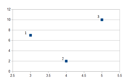
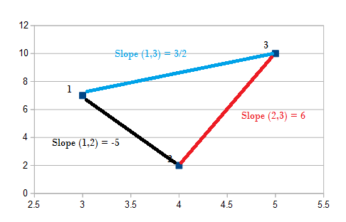
To start, use the slope formula (from elementary algebra) to find the slopes for each pair. For this example there are three pairs (1,2), (1,3), (2,3), so using the slope formula (y2 – y1) / (x2 – x1):
- 1st. Slope (1,2) = (2-7)/(4-3) = -5/1 = -5
- 2nd. Slope (1,3) = (10-7)/(5-3) = 3/2
- 3rd. Slope (2,3) = (10-4)/(5-4) = 6/1 = 6

Pairwise Independent / Mutually Independent
What is “Pairwise Independent”?
Pairwise independence means that any two events in a collection of events are independent. In other words, the occurrence of one event in a collection of events does not affect the probability of the occurrence of any other event in the collection. While every collection of mutually independent random variables is pairwise independent, some pairwise independent collections are not mutually independent. Pairwise independent random variables with finite variance are uncorrelated.
In simpler terms, within a pairwise independent probability space, the likelihood of two events occurring simultaneously is equal to the product of their individual probabilities.
Consider this example of a pairwise independent probability space:
Suppose X and Y are two random variables representing the outcomes of flipping a coin twice. The probability space for X and Y includes {HH, HT, TH, TT}, where HH denotes both coins landing heads, HT indicates the first coin lands heads and the second tails, and so on. The probability of X and Y being independent equals the product of the individual probabilities of X and Y. With both X and Y having a 1/2 probability of landing heads, The combined probability of X and Y both being heads is 1/4, which equals the product of their individual probabilities. Thus, X and Y are pairwise independent random variables.
Pairwise independent probability spaces are valuable in probability theory because they enable predictions about event likelihoods. For instance, knowing that two random variables are pairwise independent allows us to multiply their probabilities to determine the likelihood of both variables occurring.
What is Mutually Independent?
Events A, B, and C are mutually independent if they are pairwise independent:
- P(A ∩ B) = P(A) × P(B) and…
- P(A ∩ C) = P(A) × P(C) and…
- P(B ∩ C) = P(B) × P(C)
And: P(A ∩ B ∩ C) = P(A) × P(B) × P(C), which is stating that their probabilities, when multiplied together, is also the probability of the intersection of the three events.
By definition, mutually independent events are also pairwise independent. But a set of events that is pairwise independent isn’t automatically mutually independent. They must also meet the condition P(A ∩ B ∩ C) = P(A) × P(B) × P(C).
Example Problem
Question: You toss a fair coin twice. The possible events are:
- Both tosses give the same outcome (HH or TT).
- The first toss is a heads (HT HH).
- The second toss is heads (TH HH).
Are the events mutually independent?
Answer: What the question is really asking is: do these events fit the definition stated above (right under What is Mutually Independent?. The definition states that the following must be true:
P(A ∩ B ∩ C) = P(A) × P(B) × P(C)
So, we need to figure out a few probabilities first from the given information.
P(event 1), P(event 2), and P(3). You have four possible outcomes (HH, TT, TH, HT) so the probability of each pair happening is 0.25. This would make the probabilities of the events 1,2, and 3:
- Both tosses give the same outcome (HH or TT) = 1/4 + 1/4 = 1/2.
- The first toss is a heads (HT HH) = 1/4 + 1/4 = 1/2..
- The second toss is heads (TH HH) = 1/4 + 1/4 = 1/2..
Multiply the probability of events together: P(1) * P(2) * P(3) = 1/2 * 1/2 * 1/2 = 1/8. P(1 ∩ 2) = P(1 ∩ 3) = P(2 ∩ 3) = 1/4.
This is because HH is the only event that intersects (a 1 out of 4 probability). If you have trouble figuring out intersections, a Venn diagram is always a good idea. the following diagram should help you see that HH is the intersection for all three probabilities:
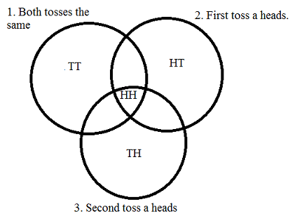
This also gives us P(1 ∩ 2 ∩ 3 ∩) = 1/4. Now you can compare the two:
- P(1 ∩ 2 ∩ 3) = P(1) × P(2) × P(3)
- 1/8 ≠ 1/4
These are not equal, so the events are not mutually independent.
Pairwise statistics
These are statistics calculated from pairs of observations. In other words, you form pairs of observations and then find a statistic of interest, like a mean or standard deviation.
References
Rosenbaum, P. Exact Confidence Intervals for Nonconstant Effects by Inverting the Signed Rank Test. The American Statistician, May 2003, Vol. 57, No. 2 Retrieved October 8, 2016 from here. url: http://stat.wharton.upenn.edu/~rosenbap/offsetEdit.pdf