Probability and Statistics > Multivariate Analysis
What is Multivariate Analysis?
Multivariate analysis is used to study more complex sets of data than what univariate analysis methods can handle. This type of analysis is almost always performed with software (i.e. SPSS or SAS), as working with even the smallest of data sets can be overwhelming by hand.
Multivariate analysis can reduce the likelihood of Type I errors. Sometimes, univariate analysis is preferred as multivariate techniques can result in difficulty interpreting the results of the test. For example, group differences on a linear combination of dependent variables in MANOVA can be unclear. In addition, multivariate analysis is usually unsuitable for small sets of data.
There are more than 20 different ways to perform multivariate analysis. Which one you choose depends upon the type of data you have and what your goals are. For example, if you have a single data set you have several choices:
- Additive trees, multidimensional scaling, cluster analysis are appropriate for when the rows and columns in your data table represent the same units and the measure is either a similarity or a distance.
- Principal component analysis (PCA) decomposes a data table with correlated measures into a new set of uncorrelated measures.
- Correspondence analysis is similar to PCA. However, it applies to contingency tables.
Although there are fairly clear boundaries with one data set (for example, if you have a single data set in a contingency table your options are limited to correspondence analysis), in most cases you’ll be able to choose from several methods.

Click on a topic to read about specific types of multivariate analysis:
- Additive Tree.
- Canonical Correlation Analysis.
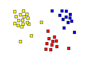
- Cluster Analysis.
- Correspondence Analysis / Multiple Correspondence Analysis.
- Factor Analysis.
- Generalized Procrustean Analysis.
- Homogeneity of Covariance
- Independent Component Analysis.
- MANOVA.
- Multidimensional Scaling.
- Multiple Regression Analysis.
- Partial Least Square Regression.
- Principal Component Analysis / Regression / PARAFAC.
- Redundancy Analysis.
Related:
Independent Component Analysis
Independent component analysis is used in statistics and signal processing to express a multivariate function by its hidden factors or subcomponents. These component signals are independent non-Gaussian signals, and the intention is that these independent sub-components accurately represent the composite signal.
The ‘cocktail party problem‘ is an often cited example of independent component analysis at work. Suppose you have a loud cocktail party, with many conversations going on in the same room. Now suppose you have a number of microphones located at various locations throughout the room, picking up the sound data. With no prior knowledge of the speakers, can you separate the signal from each microphone (in each case, a composite of all the noise in the room) into its component parts, i.e., each speakers voice?
You can do a surprisingly good job, assuming you have enough observation points. If there are N sources of noise (N guests, for example) you will need N microphones in order to fully determine the original signals.
Assumptions in Independent Component Analysis.
Independent component analysis only works if the sources are non-Gaussian (i.e. they have non-normal distributions), and so that is one of the first assumptions you make if you use this analysis on a multivariate function. Since you are attempting to break the function down into independent components, you’re also making the assumption that the original sources were in fact independent.
Mixing Effects in Independent Component Analysis
There are three principles of mixing signals which make up the foundation for independent component analysis.
- Mixing signals involves going from a series of independent signals to a series of signals that is dependent. Although your source signals are all independently generated, the composite signals are all made from the same source signals, and so cannot be independent of each other.
- Although our source signals are non-Gaussian (by the assumption we made to begin with), the composite signals are in fact Gaussian (normally distributed). This is by the Central Limit Theorem, which tells us the probability distribution function of the sum of independent variables with finite variance (like our signals) will tend toward the Gaussian distribution.
- The complexity of a signal mixture must always be greater than, or equal to, the complexity of its simplest source signal.
These three principles form the foundation for Independent Component Analysis.
Independent Component Analysis: References
Hyvärinen, Aapo. What is Independent Component Analysis? Retrieved from https://www.cs.helsinki.fi/u/ahyvarin/whatisica.shtml on April 10, 2018
Hyvärinen, Karhunen, & Oja. (2001). Independent Component Analysis. Wiley Interscience.
Ng, Andrew. CS 229 Lecture Notes: Independent Component Analysis. Retrieved from http://cs229.stanford.edu/notes/cs229-notes11.pdf on April 10, 2018
Stone, James. Independent Component Analysis. Encyclopedia of Statistics in Behavioral Science, Volume 2, pp. 907–912
Retrieved from https://pdfs.semanticscholar.org/6cdc/d22d69479c6c19f1583a281a95bc4029631e.pdf on April 10, 2018
Other References
Beyer, W. H. CRC Standard Mathematical Tables, 31st ed. Boca Raton, FL: CRC Press, pp. 536 and 571, 2002.
Dodge, Y. (2008). The Concise Encyclopedia of Statistics. Springer.
Kotz, S.; et al., eds. (2006), Encyclopedia of Statistical Sciences, Wiley.
Vogt, W.P. (2005). Dictionary of Statistics & Methodology: A Nontechnical Guide for the Social Sciences. SAGE.