The Bisection Method is used to find the root (zero) of a function. It works by successively narrowing down an interval that contains the root. You divide the function in half repeatedly to identify which half contains the root; the process continues until the final interval is very small. The root will be approximately equal to any value within this final interval.
When working with the bisection method:
- Take an interval [a, b] where f(a) and f(b) have opposite signs,
- Find the midpoint of [a, b],
- Determine whether the root is within [a, (a + b)/2] or [(a + b)/2, b].
- Repeat steps 1 through 3 until the interval is small enough.
The Bisection Method & Intermediate Value Theorem
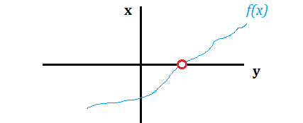
The bisection method is an application of the Intermediate Value Theorem (IVT). As such, it is useful in proving the IVT. The IVT states that suppose you have a line segment (between points a and b, inclusive) of a continuous function, and that function crosses a horizontal line. Given these facts, then the intersection of the two lines—point x—must exist.
Example—Solving the Bisection Method
Example Question: Find the 3rd approximation of the root of f(x) = x4 – 7 using the bisection method.
Step 1: Find an appropriate starting interval. This is usually an educated guess. You want an interval where the function values change sign. You can do this in three main ways:
- Plug in a few values of x or
- Look at a graph,
You could also set the equation to 0 and solve, but this may be very challenging for more complicated functions. For this example question, let’s assume the function is too challenging to solve for 0 and let’s look at a graph instead (created with Desmos):
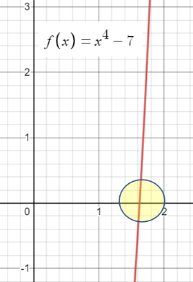
Let’s try [1, 2] as the starting interval.
Step 2: Plug in the two endpoints plus the midpoint into the function:
- f(x) = 14 – 7 = -6
- f(x) = 1.54 – 7 = -2
- f(x) = 24 – 7 = 9
The next interval for the approximation is chosen based on the results for these first three inputs. The function changes sign between my midpoint of 1.5 and the right endpoint of 2. So my “New Interval” is going to be [1.5, 2] with a new midpoint of 1.75.
Putting these into a table of values for three iterations gives:
| f(left) | f(mid) | f(right) | New Interval | Midpoint |
| f(1) = -6 | f(1.5) = -2 | f(2) = 9 | (1.5, 2) | 1.75 |
| f(1.5) = -2 | f(1.75) = 2.4 | f(2) = 9 | (1.5, 1.75) | 1.625 |
| f(1.5) = -2 | f(1.625) = -.03 | f(1.75) = 2.4 | (1.625, 1.75) | 1.6875 |
Step 3: Plug the value from Step 2 into the function. The value of the function at x is approximately 1.6875. The fourth approximation is off by at most ±0.0625.
Notice that each successive approximation builds off of the one preceding it. At each level in the table we calculate the new interval to be used in the next approximation.
this book is really helpful