Contents:
What is a Function of One Variable?
A function of one variable calculates one output value for one input value. For example, f(x) = 2x has one variable (x) and equals 4 for an input of 2:
- f(x) = 2x
- f(2) = 2(2) = 4
Function of One Variable Characteristics
A function of one variable has three defining characteristics:
- It’s a function (i.e. one input results in exactly one output),
- It has a single variable, like “x” or “t”.
- The functions deal with real numbers (as opposed to complex/imaginary numbers like 4i ).
Examples:
- f(x) = x2 + 5,
- f(x) = 2x + 5,
- f(t) = t3 + 9t,
- f(t) = t3 + t2t + 10.
Notice how all the examples have just one variable in the expression: either x or t. While x and t are the more common variables, you might see others. For example, in a trigonometric function like the sine function, you might see an angle (θ) instead, e.g. f(x) = sin(θ).
If you’re just starting out with calculus, you’re working with functions of one variable, even if it isn’t explicitly stated in your textbooks or by your professor. A function of one variable is the “common” function you’ll deal with, right up until you hit multivariable calculus and complex analysis.
Function of One Variable: Types
A function of one variable fits into a subset of different types. There are many dozens of different one-variable functions, but some of the more common ones you’ll come across include:
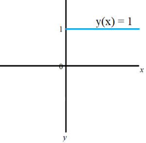
Constant functions: have the form f(x) = c, where “c” is a constant, like 5, 44, or 99.99.
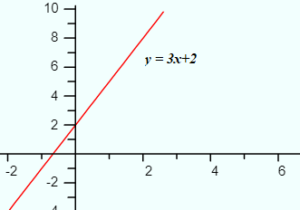
Linear Functions: functions that produce a straight line graph.
Ordinary Derivative vs. Partial
An ordinary derivative is a derivative that’s a function of one variable, like F(x) = x2. The purpose is to examine the variation of the function with respect to one variable (x, in this example). 
One of the more popular subtypes of derivatives is the partial derivative, so the “ordinary derivative” is sometimes defined in terms of a partial derivative. This isn’t strictly true (it can be a comparison with any derivative, as demonstrated below). But, for clarity, here’s the main difference between the two:
A partial derivative has more than one variable, such as F(x, y) = ax2 + by2. With a partial derivative, you hold one variable constant, in order to examine the variation of the function with respect to the other. In this example, you could hold x constant while examining y.
The term ordinary derivative is an informal term usually used to denote a “usual” or “regular” derivative, to distinguish it from other types of derivatives. For example:
- Covariant derivatives (which operate in relative complex geometrical dimensions),
- Directional derivatives. For example “This also makes our definition of the directional derivative coincide with the ordinary derivative in the one dimensional case” (Engleberg, 2018).
- Partial derivatives,
- The q-derivative (also called a Jackson derivative), a q-analog of the ordinary derivative, used in combinatorics and quantum calculus.
- Riemann derivatives—used in fractional calculus, or
- The somewhat obscure Peano derivative. For example, from Butzer et al. (1971): “Show that if the rth ordinary derivative…exists, so does the rth Peano derivative….
Many more other types of derivatives exist. So the term “ordinary” is inserted by authors just to make it clear which derivative is which.
Weak Derivative
The weak derivative uxi is an extension of the ordinary derivative to allow for the inclusion of problematic “points” that would otherwise make useful functions non-differentiable. Weak derivatives are sometimes called distributional derivatives [1].
For example, the absolute value function cannot be differentiated on the interval [-2, 2] because of a sharp corner:
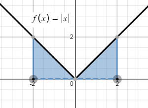
However, we can approach this problem from the backend: the function can be integrated (using integration by parts) [2]. We can then work backwards, creating a derivative that isn’t quite as “strong” as one we would have had if we could have used the usual routes for finding derivatives:
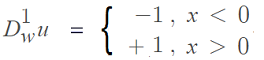
.
We could choose to include the function’s corner value at x = 0 in either interval. The choice is arbitrary and makes no difference [3]. Obviously though, this weak derivative is forced to work on a space (i.e. the problematic corner) that it shouldn’t be defined on in the classical sense. We call this forced construct a Sobolev space, named after S. L. Sobolev, who first introduced the idea of a weak derivative [4].
We can perform this backwards magic because of the Fundamental Theorem of Calculus (FTC); Like their ordinary counterparts, weak derivatives satisfy the theorem. If the ordinary derivative exists, then the weak and ordinary derivatives are equivalent.
Another Piecewise Example
The piecewise function shown in the following image has a problematic corner at x = 1, which means that the ordinary derivative cannot be found at that point:
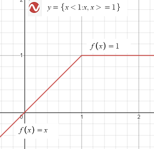
However, if the sharp corner is ignored, we can define the weak derivative:
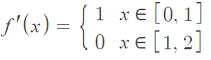
Again, the choice of which interval to put the function value at the problematic point in (the first, second, both, or none) is not relevant.
Use of the Weak Derivative for Functions of One Variable
Weak derivatives are usually used as an intermediate step towards a solution. For example, when looking for solutions to partial differential equations, it’s often easier to ask for weak derivatives and then show the solution is differentiable in the ordinary sense [5].
Weak Derivative: References
Desmos graphing calculator.
[1] Johnson, et al. (2017). When functions have no value(s): Delta functions and distributions. Retrieved July 17, 2021 from: https://math.mit.edu/~stevenj/18.303/delta-notes.pdf
[2] Jost J. (1998) Integration by Parts. Weak Derivatives. Sobolev Spaces. In: Postmodern Analysis. Universitext. Springer, Berlin, Heidelberg. https://doi.org/10.1007/978-3-662-03635-8_21
[3] Sobolev Spaces. Retrieved May 6, 2021 from: https://www.math.ucdavis.edu/~hunter/pdes/ch3.pdf
[4] Soboleva, S. L. (1979). [in Russian]. On the mixed boundary-value problems for Sobolev-type equations with variable coefficients. Tr. Semin.
[5] Weber, J. (2018). Introduction to Sobolev Spaces. Retrieved May 5, 2021 from: http://www.math.stonybrook.edu/~joa/PUBLICATIONS/SOBOLEV.pdf
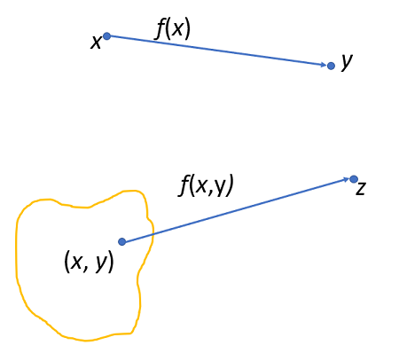
Function of Two Variables
A function of two variables
The formal definition of a function of two variables is similar to the definition for a function of one variable.
A function of two variables f(x, y) has a unique value for f for every element (x, y) in the domain D.
has two inputs (independent variables).
Many common functions have two inputs, including:
- Area of a rectangle with two sides l and w: A = lw
- Work done by force F with displacement d: W = Fd,
- Volume of a right circular cylinder with radius r and height h (V = πr2h). Note that π is a constant and doesn’t count here as a variable.
While a single variable function maps the value of one variable to another, a function of two variables maps ordered pairs (x, y) to another variable.
Notation
Notation for a function of two variables is very similar to the notation for functions of one variable. For example:
- Function on one variable: f(x) = x2
- Two variable function: f(x, y) = x2 + 2y
How to Find the Domain of a Function of Two Variables
The domain is the set of points where the function is defined. Some authors will specify the domain; Many times (especially in real life) you’ll have to figure out what makes sense.
A good starting point is to assume that the domain is all real numbers (from -∞ to ∞), then look for areas where the function doesn’t work. This is where a good knowledge of algebra will come in handy, but if you’re rusty— here are a couple of basic steps (which will catch most of the undefined areas).
Step 1: Ask yourself: Where does this make sense? If a formula is given, like A = lw, then
assume that the domain is defined for points that make sense, unless a specific domain is given. What “makes sense” will depend on the specific situation, but here are a couple of examples:
- Area only makes sense for values of length and width greater than 0.
- Volume only makes sense for positive valued inputs.
Step 2: Look for division by zero.
If a formula has x in a denominator, like this one:
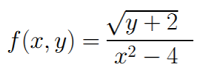
Then figure out what would make the denominator zero. The function will be undefined at those points. For this particular formula, the domain is all real numbers (-&infin, ∞) except for x = ±2
Step 2: Look for values that will make quantities under a square root negative. For example:
f(x, y) = √(9 – x2 – y2)
If (x2 – y2) equals anything less than 9, then the value under the square root becomes negative. Therefore, the domain here is all reals except where (x2 – y2) ≤ 9. In more formal notation, you can write that as:
The domain of f(x, y) = {(x, y) ∈ ℝ | x2 – y2 ≤ 9}
Where
- ℝ (doublestruck R) = the set of all real numbers,
- ∈ = “is in the set of”.
Function of One Variable: References
Ash, J. A Characterization of the Peano Derivative. Transactions of the American Mathematical Society. Volume 149, June, 1970
Butzer, P. et al. (1971). Fourier Analysis and Approximation.
Engleberg, S. (2018). Random Signals and Noise: A Mathematical Introduction.
Larson, R. & Edwards, B. (2009). Calculus. Cengage Learning.
Nave, C. (2016). The Derivative. Retrieved December 30, 2019 from: http://hyperphysics.phy-astr.gsu.edu/hbase/deriv.html
Oldham, K. et al. (2008). An Atlas of Functions: with Equator, the Atlas Function Calculator 2nd Edition. Springer.