Contents:
- Definition of a Probability Distribution
- Probability Distribution Table Definition
- A to Z List of Distributions
What is a Probability Distribution?
A probability distribution tells you what the probability of an event happening is. Probability distributions can show simple events, like tossing a coin or picking a card. They can also show much more complex events, like the probability of a certain drug successfully treating cancer.
There are many different types of probability distributions in statistics including:
- Basic probability distributions which can be shown on a probability distribution table.
- Binomial distributions, which have “Successes” and “Failures.”
- Normal distributions, sometimes called a Bell Curve.
The sum of all the probabilities in a probability distribution is always 100% (or 1 as a decimal).
Ways of Displaying Probability Distributions
Probability distributions can be shown in tables and graphs or they can also be described by a formula. For example, the binomial formula is used to calculate binomial probabilities.
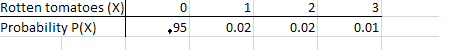
The following table shows the probability distribution of a tomato packing plant receiving rotten tomatoes. Note that if you add all of the probabilities in the second row, they add up to 1 (.95 + .02 +.02 + 0.01 = 1).
The following graph shows a standard normal distribution, which is probably the most widely used probability distribution. The standard normal distribution is also known as the “bell curve.” Lots of natural phenomenon fit the bell curve, including heights, weights and IQ scores. The normal curve is a continuous probability distribution, so instead of adding up individual probabilities under the curve we say that the total area under the curve is 1.
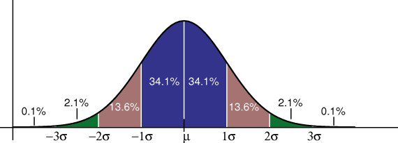
Note: Finding the area under a curve requires a little integral calculus, which you won’t get into in elementary statistics. Therefore, you’ll have to take a leap of faith and just accept that the area under the curve is 1!
Probability Distribution Table
A probability distribution table links every outcome of a statistical experiment with the probability of the event occurring. The outcome of an experiment is listed as a random variable, usually written as a capital letter (for example, X or Y). For example, if you were to toss a coin three times, the possible outcomes are:
TTT, TTH, THT, HTT, THH, HTH, HHT, HHH
You have a 1 out of 8 chance of getting no heads at all if you throw TTT. The probability is 1/8 or 0.125, a 3/8 or 0.375 chance of throwing one head with TTH, THT, and HTT, a 3/8 or 0.375 chance of throwing two heads with either THH, HTH, or HHT, and a 1/8 or .125 chance of getting three heads.
The following table lists the random variable (the number of heads) along with the probability of you getting either 0, 1, 2, or 3 heads.
| Number of heads (X) | Probability P(X) |
| 0 | 0.125 |
| 1 | 0.375 |
| 2 | 0.375 |
| 3 | 0.125 |
Probabilities are written as numbers between 0 and 1; 0 means there is no chance at all, while 1 means that the event is certain. The sum of all probabilities for an experiment is always 1, because if you conduct and experiment, something is bound to happen! For the coin toss example, 0.125 + 0.375 + 0.375 + 0.125 = 1.
Need help with a homework question? Check out our tutoring page!
More complex probability distribution tables
Of course, not all probability tables are quite as simple as this one. For example, the binomial distribution table lists common probabilities for values of n (the number of trials in an experiment).

The more times an experiment is run, the more possible outcomes there are. the above table shows probabilities for n = 8, and as you can probably see — the table is quite large. However, what this means is that you, as an experimenter, don’t have to go through the trouble of writing out all of the possible outcomes (like the coin toss outcomes of TTT, TTH, THT, HTT, THH, HTH, HHT, HHH) for each experiment you run. Instead, you can refer to a probability distribution table that fits your experiment.
Check out our YouTube channel for more stats help and tips!
List of Statistical Distributions
Jump to A B C D E F G H I J K L M N O P R S T U V W Y Z.
Click any of the distributions for more information.
A
- Absolutely Continuous Distribution.
- Alpha Distribution.
- Amoroso Distribution.
- Analytic Distribution.
- Arcsine Distribution.
- Arfwedson Distribution.
- Argus Distribution.
- Array Distribution.
- Balding-Nichols Distribution.
- Bates Distribution.
- Bathtub-Shaped Distribution.
- Beckmann Distribution.
- Bell Shaped Distribution.
- Benford Distribution: Definition, Examples.
- Benini Distribution.
- Bernoulli Distribution.
- Beta Binomial Distribution.
- Beta Distribution.
- Beta Exponential Distribution.
- Beta Geometric Distribution (Type I Geometric).
- Beta Prime Distribution.
- Bingham Distribution.
- Binomial Distribution.
- Bimodal Distribution.
- Birnbaum-Saunders Distribution
- Bipolar Distribution.
- Bivariate Distribution.
- Bivariate Normal Distribution.
- Bivariate Poisson Distribution.
- Borel Distribution.
- Bounded Distribution.
- Bradford Distribution.
- Burr Distribution.
- Cantor Distribution.
- Categorical Distribution.
- Cauchy Distribution.
- Chi Distribution.
- Chi-Bar-Squared Distribution.
- Circular Distribution.
- Compound Probability Distribution.
- Compound Poisson Distribution (Pollaczek–Geiringer).
- Conjugate Prior Distribution.
- Continuous Joint Distribution.
- Continuous Probability Distribution.
- Conway-Maxwell-Poisson Distribution.
- Copula Distributions.
- Cosine Distribution.
- Cramp Function Distribution.
- Cumulative Frequency Distribution.
- Cumulative Distribution Function.
- Dagum Distribution.
- Davis Distribution.
- Degenerate Distribution.
- Delaporte distribution.
- Delta Distribution.
- De Moivre Distribution.
- Directional Distribution.
- Dirichlet Distribution.
- Discrete Probability Distribution.
- Easy Distribution.
- Elliptical Distribution.
- Empirical Distribution Function.
- Erlang Distribution.
- Eulerian Distribution.
- Exponential Dispersion Models.
- Exponential Distribution.
- Exponential-Type Distribution.
- Exponential-Logarithmic Distribution.
- Exponential Power Distribution.
- Exponentiated Exponential Distribution.
- Exponentiated Weibull Distribution.
- Extreme Value Distribution.
- F Distribution.
- Factorial Distribution.
- Fat Tail Distribution.
- Ferreri Distributions
- Fisher Z Distribution.
- Fisk Distribution.
- Flory-Schulz Distribution.
- Folded Normal / Half Normal Distribution.
- G-and-H Distribution.
- Gamma Distribution.
- Gamma-Normal Distribution.
- Gamma Poisson Distribution.
- Generalized Beta Distribution.
- Generalized Error Distribution.
- Generalized Gamma Distribution.
- Geometric Distribution.
- Ghosh distribution.
- GIG Distribution.
- Gompertz Distribution.
- Gompertz-Makeham Distribution.
- Gram-Charlier Distribution.
- Grand Unified Distribution.
- Half-Cauchy Distribution.
- Half-Logistic Distribution.
- Halphen Distribution.
- Hansmann’s Distributions.
- Hard Distribution.
- Helmert’s Distribution.
- Hermite Distribution.
- Heavy Tailed Distribution.
- Holtsmark Distribution.
- Hurdle Distribution.
- Hyperbolic Secant Distribution.
- Hyperexponential Distribution.
- Hypergeometric Distribution.
- Hyperbolic Distribution.
- Laha Distribution.
- Landau Distribution.
- Laplace Distribution.
- Lévy Distribution.
- Lifetime Distributions.
- Linear exponential family.
- Lindley Distribution.
- Location-Scale Family of Distributions.
- Logarithmic Distribution.
- Loglinear model / distribution.
- Lognormal Distribution.
- Lomax Distribution.
- Long Tail Distribution.
- Marginal Distribution.
- Mielke’s Beta-Kappa Distribution.
- Mixture Distribution.
- Modified Geometric Distribution.
- Multimodal Distribution.
- Multinomial Distribution.
- Multivariate Distribution: Definition
- Multivariate Gamma Distributions
- Multivariate Normal Distribution.
- Muth Distribution.
- Nakagami Distribution.
- Negative Binomial Distribution.
- Negative Hypergeometric Distribution.
- Non-Central Distribution.
- Noncentral Beta Distribution.
- Noncentral Chi-Squared distribution.
- Non-Parametric Distribution.
- Normal Distribution.
- Parabolic Distribution.
- Parametric Distribution.
- Pareto Distribution.
- Pearson Distribution.
- PERT Distribution.
- Phase Type Distribution.
- Pólya Distribution.
- Poisson Distribution.
- Power Function Distribution.
- Power Law Distribution.
- Power Series Distributions.
- Rademacher Distribution.
- Raised cosine distribution.
- Ratio distribution.
- Rayleigh Distribution.
- Reciprocal Distribution.
- Relative Frequency Distribution.
- Rician Distribution.
- Robust Soliton Distribution.
- Rutherford distribution.
- Semicircle Distribution.
- Severity Distribution.
- Sibula Distribution.
- Sine Distribution.
- Singular Distribution.
- Skellam Distribution (Poisson Difference Distribution).
- Skewed Distribution.
- Slash Distribution.
- Smooth distribution.
- Special Distribution
- Stable Distribution.
- Standard Power Distribution & U Power Distribution.
- Stuttering Poisson Distribution.
- Survival Distribution.
- Symmetric Distribution.
- T Distribution.
- Tine Distribution.
- Trapezoidal Distribution.
- Triangular Distribution.
- Truncated Normal Distribution.
- Tukey Lambda Distribution.
- Tweedie Distribution.
- Wallenius Distribution.
- Waring Distribution.
- Weibull Distribution.
- Wilson-Hilferty Distribution.
- Wrapped Normal Distribution.
- Wishart Distribution.
See also:
G-and-h distribution
The g-and-h distribution is a continuous probability distribution that was developed by John Tukey in 1977. It is a two-parameter distribution, with the parameters g and h. The g-and-h distribution is a generalization of the gamma distribution, and it can be used to model a variety of data sets, including data sets that are skewed or have heavy tails.
The g-and-h distribution is defined as follows:
f(x) = g h x^(g – 1) exp(-h x) / Gamma(g),
where:
- f(x) is the probability density function of the g-and-h distribution.
- x is the random variable.
- g and h are the parameters of the distribution.
- Gamma(g) is the gamma function.
The g-and-h distribution has a number of properties that make it a useful tool for modeling data. These properties include:
- The g-and-h distribution is flexible, and it can be used to model a variety of data sets.
- The g-and-h distribution is robust, and it is not sensitive to outliers.
- The g-and-h distribution is easy to estimate, and there are a number of software packages that can be used to estimate the parameters of the distribution.
The g-and-h distribution is a useful tool for a variety of applications, including:
Statistical modeling: The g-and-h distribution can be used to model a variety of data sets, including data sets that are skewed or have heavy tails.
Risk analysis: The g-and-h distribution can be used to model the risk of rare events, such as natural disasters or financial crises.
Decision making: The g-and-h distribution can be used to make decisions under uncertainty, such as decisions about how to allocate resources or how to invest money.
Overall, the g-and-h distribution is a versatile and powerful tool for modeling data. It is easy to estimate and use, and it can be used to model a variety of data sets.
Tine Distribution
What is the Tine Distribution?
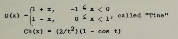
The little known Tine distribution , sometimes called the symmetric triangular distribution, is a continuous probability distribution shaped like a triangle. It is also called Simpson’s distribution, after Thomas Simpson (1710-1761) who is thought to be the first to suggest the distribution [1]. The distribution was not mentioned in the literature again until R. Schmidt’s 1934 article in the Annals of Mathematical Statistics [2]. Schmidt was the first to call it the “tine distribution” (a tine is a slender projecting point).
The tine distribution made an entry in the Index to the 1958 Distributions of Mathematical Statistics [3] as:
Rinne [3] defines the Tine distribution as the distribution of two independent and identically distributed (i.i.d.) uniform variables (i.e., the convolution of two uniform distributions):
X1, X2 iid∼ UN(a, b) ⇒ X = X1 + X2 ∼ TS(2 a + b, b).
A convolution is an operation on two functions (f and g) that produces a third function (), which expresses how the shape of one function is modified by the other.
The distribution isn’t widely known. In fact, if you try and Google “tine Distribution” you’ll be redirected (at the time of writing) to pages on “time distribution” instead. It’s also not often used (most likely because it isn’t well known!), but there are a few specific use cases. For example, this Google patent for an “Authentication device and authentication method” includes the tine distribution as a threshold measure.
The threshold value determination part 22 is Mahalanobis prescribed | regulated by the Mahalanobis distance prescribed | regulated by the mean value and the standard deviation of a person distribution, and the average value and standard deviation of a tine distribution. To match the distance, the threshold value Xth is determined.
Google patent for an authentication device
Note that the patent makes reference to a “person distribution” which is most likely the author’s name for the distribution of biometric authentication data.
References
[1] Rinne, H. Location–Scale Distributions Linear Estimation and Probability Plotting Using MATLAB. Online: http://geb.uni-giessen.de/geb/volltexte/2010/7607/pdf/RinneHorst_LocationScale_2010.pdf
[2] Haight, F. (1958). Index to the Distributions of Mathematical Statistics. National Bureau of Standards Report.
[3] Schmidt, R. Statistical Analysis of One-Dimensional Distributions. Annals of Mathematical Statistics. 5:33. 1934