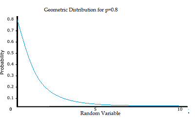
What is a Geometric Distribution?
The geometric distribution represents the number of failures before you get a success in a series of Bernoulli trials.
PDF for the Geometric Distribution
This discrete probability distribution is represented by the probability density function:
f(x) = (1 − p)x − 1p
For example, you ask people outside a polling station who they voted for until you find someone that voted for the independent candidate in a local election. The geometric distribution would represent the number of people who you had to poll before you found someone who voted independent. You would need to get a certain number of failures before you got your first success.
If you had to ask 3 people, then X = 3; if you had to ask 4 people, then X=4 and so on. In other words, there would be X – 1 failures before you get your success.
If X = n, it means you succeeded on the nth try and failed for n-1 tries. The probability of failing on your first try is 1 – p. For example, if p = 0.2 then your probability of success is .2 and your probability of failure is 1 – 0.2 = 0.8. Independence (i.e. that the outcome of one trial does not affect the next) means that you can multiply the probabilities together. So the probability of failing on your second try is (1 – p)(1 – p) and your probability of failing on the nth-1 tries is (1 – p)n – 1. If you succeeded on your 4th try, n = 4, n – 1 = 3, so the probability of failing up to that point is (1 – p)(1 – p)(1 – p) = (1 – p)3.
For more examples see: 7 Real Life Examples of the Geometric Distribution
Example
Example question: If your probability of success is 0.2, what is the probability you meet an independent voter on your third try?
Inserting 0.2 as p and with X = 3, the probability density function becomes:
- f(x) = (1 − p)x − 1*p
- P(X = 3) = (1 − 0.2)3 − 1(0.2)
- P(X = 3) = (0.8)2*0.2 = 0.128.

Theoretically, there are an infinite number of geometric distributions. The value of any specific distribution depends on the value of the probability p.
Assumptions for the Geometric Distribution
The three assumptions are:
- There are two possible outcomes for each trial (success or failure).
- The trials are independent.
- The probability of success is the same for each trial.
Connection to the Geometric Series
The geometric distribution can model the number of trials up to a certain success or the number of failures until the first success. In either case, the sequence of probabilities is a geometric sequence. Infinite series, particularly the geometric series
![]()
are useful for understanding how the distribution works ( Kjos-Hanssen, 2019).
References
Beyer, W. H. CRC Standard Mathematical Tables, 31st ed. Boca Raton, FL: CRC Press, pp. 536 and 571, 2002.
Agresti A. (1990) Categorical Data Analysis. John Wiley and Sons, New York.
Kjos-Hanssen, B. (2019). Statistics for Calculus Students. Retrieved April 30, 2021 from: https://people.math.osu.edu/husen.1/teaching/530/series.pdf
Kotz, S.; et al., eds. (2006), Encyclopedia of Statistical Sciences, Wiley.
Wheelan, C. (2014). Naked Statistics. W. W. Norton & Company