Probability Distributions > Cauchy Distribution
What is a Cauchy Distribution?
The Cauchy distribution, sometimes called the Lorentz distribution, is a family of continuous probably distributions which resemble the normal distribution family of curves. While the resemblance is there, it has a taller peak than a normal. And unlike the normal distribution, it’s fat tails decay much more slowly.
The Cauchy distribution is well known for the fact that it’s expected value and other moments do not exist. The median and mode do exist. And for the Cauchy, they are equal. Together, they tell you where the line of symmetry is. However, the Central Limit theorem doesn’t work for the limiting distribution of the mean. In sum, this distribution behaves so abnormally it’s sometimes considered the Hannibal Lecter of distributions.
- “It’s best known as a pathological case” (Segura et. al, 2004).
- It is “perhaps more curious than useful” (Marshall, 2007).
Uses
So, if it doesn’t work so well, why study it at all? While it’s often used as an example of the “opposite” of how distributions should work, it does have a few practical applications. For example:
- It’s a popular distribution for robustness studies.
- It models the ratio of two normal random variables.
- It models polar and non-polar liquids in porous glasses (Stapf et. al, 1996)
- In quantum mechanics, it models the distribution of energy of an unstable state (Grewel & Andrews, 2015).
Defining the Distribution
The Cauchy distribution has two main parts: a scale parameter (λ) and a location parameter (x0).
- The location parameter (x0) tells us where the peak is.
- The scale parameter is half the width of the PDF at half the maximum height.
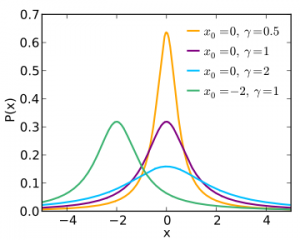
In other words, the location parameter x0 shifts the graph along the x-axis and the scale parameter λ results in a shorter or taller graph. The smaller the scale parameter, the taller and thinner the curve. In the image below, the smaller value for lambda (0.5) gives the tallest and thinnest graph, shown in orange.

The standard Cauchy distribution (shown in purple on the above graph) has a location parameter of 0 and a scale parameter of 1; the notation for the standard distribution is X ~ Cauchy(1,0) or more simply, C(1,0).
On μ and σ
Sometimes, you might see the more recognizable μ (i.e. the mean) instead of (x0). However, as the mean doesn’t technically exist, the notation μ is best avoided because of the potential confusion. If you do use μ you should think of it as the middle of the curve (rather than the average). Lambda is about the same as the standard deviation, σ. But as the standard deviation doesn’t exist for this distribution either, you may want to avoid using σ as well.
Expected Value
If the expected value did exist, it would equal the mean, which is zero. However, the mean in a Cauchy doesn’t exist (nor do higher moments like the standard deviation and skewness). So the expected value doesn’t exist either.
Calculus can prove these properties. Basically, ∫xrf(x)d(x) don’t converge in absolute value. Therefore, there aren’t any moments.
You can find a different interpretation here.
PDF Function
The formula for the probability density function is:

This online calculator at Casio.com will calculate the PDF as well as the upper and lower CDF for a Cauchy distribution.
References:
Grewel and Andrews (2015). Kalman Filtering. John Wiley & Sons.
Krishnamoorthy (2006). Handbook of Statistical Distributions with Applications. CRC Press.
Marshall and Olkin (2007). Life Distributions. Springer Science and Business.
Segura et. al (2004). A Guide to Laws and Theorems Named After Economists. Edward Elgar publishing.
Stapf et. al (1996). Proton and deuteron field-cycling. Colloids and Surfaces: A Physicochemical and Engineering Aspects 115, 107-114.