< Probability Distributions List < Birnbaum-Saunders Distribution
Contents:
What is the Birnbaum-Saunders distribution?
The Birnbaum-Saunders distribution represents the distribution of lifetimes for components under certain wear conditions. This unimodal distribution was originally formulated to model failures due to cracks, it is an example of a fatigue life distribution.
A common form of the Probability Density Function (pdf) for the Birnbaum-Saunders distribution is [1]:
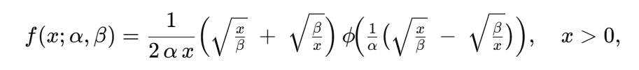
Where
- α > 0 is the shape parameter
- β > 0 is the scale parameter
- ϕ(⋅) denotes the standard normal pdf.
The distribution is a mixture distribution of an inverse Gaussian distribution and a reciprocal inverse Gaussian distribution [2]. Shapes of the distribution vary from highly skewed with long tails to almost symmetric as values for β increase [2].
There are several different variations on the formula in the literature. For example, Desmond rewrites the formula as [3]:
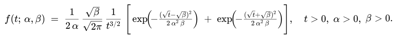
Where:
- t = time-to-failure (or crack-propagation time, etc.),
- > 0 = the shape (sometimes called the “fatigue” parameter),
- > 0 = the scale parameter (sometimes related to an initial crack size or threshold).
This is equivalent to more common Birnbaum–Saunders pdf you may see in other references. In his paper, Desmond showed that you can relax certain assumptions of the original Birnbaum–Saunders derivation and still arrive at a distribution of the same general form.
Rieck and Nedelman [4] presented a log-linear model for the distribution, applicable to accelerated life-testing. The model treats each lifetime Ti as TiBS (α, Βi), with fixed shape parameter α and scale parameter Βi, satisfying the equation
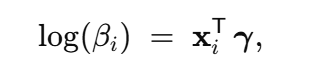
In short, their model is just the Birnbaum–Saunders distribution with scale parameter β modeled as an exponential function of covariates. this gives us a convenient and easily understood way to model lifetime data.
If a data set that is thought to be Birnbaum–Saunders distributed, the parameters’ values are best estimated by maximum likelihood [5], although a Jackknife estimator is a possibility [6].
Other types of fatigue life distribution
Various fatigue life distributions exist, each with their own pros and cons. While the Birnbaum-Saunders distribution is commonly known as “the”
fatigue life distribution [1], there are some other types commonly used to model fatigue life data. They include:
- Normal distribution: Often used for modeling fatigue life data, the normal distribution is symmetric and relatively easy to comprehend and apply. It enables predictions about a product’s fatigue life. However, it may be inaccurate for specific types of fatigue life data, such as highly skewed data or data with a long tail.
- Log-normal distribution: This right-skewed distribution is frequently used to model highly skewed fatigue life data. While it offers greater accuracy than the normal distribution for this kind of data, it can be more challenging to understand and use.
- Weibull distribution: This is a versatile option for modeling a wide range of fatigue life data. It generally provides better accuracy than the normal distribution for most fatigue life data types and is relatively simple to comprehend and use.
- Gompertz-Makeham distribution: This two-parameter distribution is commonly used for modeling fatigue life data characterized by a decreasing failure rate. Although it offers higher accuracy than the normal distribution for such data, it can be more difficult to understand and use.
The selection of a fatigue life distribution depends on the data being modeled and the required accuracy level. Generally, the normal distribution is suitable for non-highly skewed fatigue life data, while the log-normal or Weibull distribution is appropriate for highly skewed data. The Gompertz-Makeham distribution is an ideal choice for fatigue life data characterized by a decreasing failure rate.
Some key features of the different types of fatigue life distribution:
| Distribution | Shape | Symmetry | Mean | Variance |
|---|---|---|---|---|
| Normal distribution | Bell-shaped | Symmetric | μ | σ2 |
| Lognormal distribution | Right-skew | Asymmetrical | μ+σln(z) | σ2(ln(z))2 |
| Weibull distribution | Right-skew | Asymmetrical | βΓ(α) | β2Γ(α)2 |
| Gompertz-Makeham distribution | Right-skew | Asymmetrical | μexp(βt) | μ2β2exp(2βt) |
Where:
- μ = mean
- σ = standard deviation
- α = shape parameter
- β = scale parameter
- z = random variable
- Γ = Gamma function
References
- Birnbaum, Z. W., and Saunders, S. C. (1969). A new family of life distributions, Journal of Applied Probability, 6, 319-327.
- Engineering Statistics Handbook. Fatigue Life (Birnbaum-Saunders). Online: https://www.itl.nist.gov/div898/handbook/apr/section1/apr166.htm
- Desmond, A. F. (1986). On relationship between two fatigue-life models, IEEE Transactions on Reliability, 35, 167-1 69.
- Rieck, J. R., and Nedelman, J. (1991). A log-linear model for the Birnbaum-Saunders distribution, Technometrics, 33, 51-60.
- Birnbaum, Z. W., and Saunders, S. C. (1969). Estimation for a family of life distributions with applications to fatigue, Journal of Applied Probability, 6, 328-347.
- Ahmad, I. A. (1988). Jackknife estimation for a family of life distributions, Journal of Statistical Computation and Simulation, 29, 211-223.
- NIST. Birnbaum-Saunders (Fatigue Life) Distribution. Retrieved June 8, 2023 from:https://www.itl.nist.gov/div898/handbook/eda/section3/eda366a.htm