Delta Distribution

< List of probability distributions < Delta distribution

What is a delta distribution?

The term delta distribution has at least three separate meanings: it may refer to:

• The zero-modified lognormal distribution developed by Aitchison and Brown,
• The Dirac delta distribution.
• In quantum mechanics, the delta distribution has an entirely different meaning: it is the functional δ(Φ) that associates every test function Φ(x) a number. A functional is an extension of the calculus concept of a function, where we can define quantities that are not true functions in the classical analysis sense; instead of y = f(x), the function f is determined by its action on a set of test functions Φ(x); thus, a functional associates any number f(Φ) with each test function Φ [1].

1. Zero-modified lognormal distribution

The zero-modified lognormal (delta) distribution is a mixture distribution with a positive probability of a zero observation; positive observations (i.e., non-zero observations) have a log-normal distribution. The delta distribution is a special case of a zero-modified distribution.

The probability density function (pdf) h(y;μ,σ,p) is:

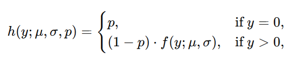
Where

• $p$ is the probability of observing a zero,
• f(y;μ,σ) is the probability density function of a lognormal distribution, which is:

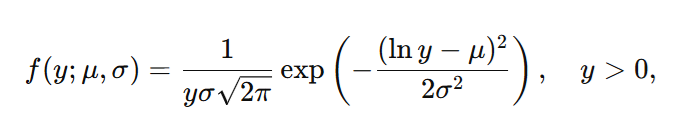
• $\mu$ and σ are the mean and standard deviation of the natural logarithm of the variable $y$,
• h(y;μ,σ,p) accounts for the probability of zero observations and the lognormal distribution of positive observations.

Note that the standard deviation (σ) and mean (μ) refer to the lognormal part of the mixture distribution.

Aitchinson and Brown [2] developed the “delta distribution” or zero-modified lognormal distribution to model economic data, although some researchers have applied the delta distribution to environmental data [3]. When sample data are non-negative and right-skewed, the minimum variance unbiased estimator (MVUE) of the delta distribution’s has been suggested as an alternative to the sample mean [4].

2. Dirac Delta Function / Distribution

The Dirac delta function isn’t a true “function” at all. The Dirac delta is an element of a set of mathematical objects called distributions – so the function is more aptly named a “delta distribution.”

The delta distribution describes real-world phenomena that can’t be described by regular functions. It  is widely used to describe analysis of concrete models (equations), signal transfer, signal boost, in picture detection and texture removal of pictures.  It is also used in a wide variety of natural sciences to describe white noise, the set of all sounds, or white light, the set of all light frequencies, or black holes, or delta shocks (from phenomenon such as earthquakes or tsunamis) [5].

Many “generalized” functions in real-world phenomena such as these can’t be described by true mathematical functions. Dirac’s delta models a unit impulse that passes through a system in an instant and is most often found in classical and quantum mechanics.

The Dirac has a unique property that sets it apart from other functions. While its value is zero for all inputs except at x = 0, where it becomes infinite, it disappears on any open interval that does not contain x = 0.

Its namesake, Paul Dirac, was a pioneering nuclear physicist who recognized the function’s potential and its usefulness within these disciplines. Despite its specific properties, the Dirac function remains an important and versatile component of many scientific and mathematical applications.

3. Delta distribution and generalized functions

The Dirac delta distribution (function) is sometimes called “the” generalized function (or “the” generalized distribution). Generalized functions are, perhaps confusingly, a new way of defining a function with no values. You can think of it as an updated limit (from calculus); but instead of measuring an interval around a point, takes a carefully defined test function (one that models the phenomena sufficiently well) and returns real numbers for analysis.

The definition is written as

f is a rule, that given a test function φ(x) returns a number f {φ)².

As an example, let’s say you wanted to create a function that represented the force of the impact of the meteor that wiped out the dinosaurs. The only value in that function would be at the exact moment the meteor hit the Earth. We can call that t = 0. At t = 0, the function has a value approximately equivalent to 10 billion atomic bombs. The impact would have been over in a flash. Every other value for “t” would equal zero. Up until the introduction of generalized functions, it wasn’t possible to use functions to describe this process, or any others like it.

References

1. Muller-Kirsten, H. (2012). Introduction To Quantum Mechanics: Schrodinger Equation And Path Integral (Second Edition). World Scientific.
2. Aitchinson, J. and Brown, J. (1957). The lognormal distribution. Cambridge University Press, pages 87-99.
3. Owen, W. & DeRouen, T. (1980). Estimation of the mean for lognormal data containing zeroes and left-censored values with applications to the measurement of worker exposure to air contaminants. Biometric, 36:707-719.
4. Syrjala, S. Critique on the use of the delta distribution for the analysis of trawl survey data. ICES Journal of marine science. 57:831-842. 2000.
5. Stevan Pilipovic, Djurdjica Takaci. On the delta distribution: Historical remarks, Visualization of delta sequences. Teaching mathematics and statistics in sciences. Retrieved June 27, 2022 from: http://citeseerx.ist.psu.edu/viewdoc/download?doi=10.1.1.362.8837&rep=rep1&type=pdf