Probability Distributions > Uniform Distribution
Contents:
- What is a uniform distribution?
- General formula and properties
- Finding probabilities: Examples
- Continuous vs. discrete uniform distribution
What is a Uniform Distribution?
A uniform distribution, also called a rectangular distribution, is a probability distribution that has constant probability. The distribution is defined by two parameters:
- minimum, a.
- maximum, b.
In between the minimum and maximum, the distribution has the same function values (i.e., equal y-values) for each input of x. The following graph shows the distribution with a = 1 and b = 3: 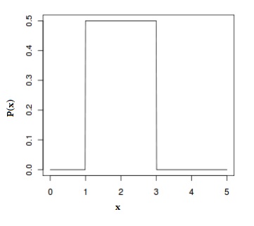 Like all probability distributions for continuous random variables, the area under the graph of a random variable is always equal to 1. In the above graph, the area is: A = l x h = 2 * 0.5 = 1. Note: In actuarial science, the uniform distribution is called the de Moivre distribution.
General formula and properties
The general formula for the probability density function (pdf) for the uniform distribution is:
f(x) = 1/ (B-A) for A≤ x ≤B.
- A is the location parameter: The location parameter tells you where the center of the graph is.
- B” is the scale parameter: The scale parameter stretches the graph out on the horizontal axis.
Note: The A and B here aren’t to be confused with lowercase (a,b), which is an open interval.
CDF
The uniform distribution doesn’t always look like a rectangle. A special case, the uniform cumulative distribution function, adds up all of the probabilities (in the same way a cumulative frequency distribution adds probabilities) and plots the result, which is a linear graph and not a rectangle: 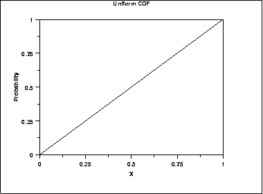
Expected value and variance
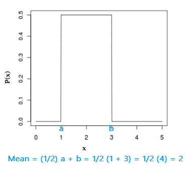
The expected value (or mean) of a uniform random variable X is:
E(X) = (1/2) (a + b)
or, equivalently:
E(X) = (b + a) / 2.
For example, with a = 1 and b = 3, the expected value is E(X) = (1 + 3) / 2 = 2.
The variance of a uniform random variable is:
Var(x) = (1/12)(b-a)2
For the above image, the variance is (1/12)(3 – 1)2= 1/12 * 4 = 1/3.
Finding probabilities: Examples
Example question #1: The average amount of weight gained by a person over the winter months is uniformly distributed from 0 to 30lbs. Find the probability a person will gain between 10 and 15lbs during the winter months. 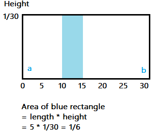
- Find the height of the distribution. The area under a probability distribution is always 1. As there are 30 units (from zero to 30), then the height is 1/30.
- Find the width of the “slice” of the distribution mentioned in the question. Do this by subtracting the biggest number (b) from the smallest (a), to get b – a = 15 – 10 = 5.
- Multiply the width (Step 2) by the height (Step 1) to get: Probability = 5 * 1/30 = 5/30 = 1/6.
Example Question 2: Find P(X≤10) for the above question. This is asking you to find the probability that the random variable X is less than 10. In other words, you want to know the probability a person will gain up to ten pounds.
- Find the width of the “box”: b – a = 10 – 0 = 10.
- Multiply the width (Step 1) by the height. We already know the height is 1/30 (from example question 1), so: 10 * 1/30 = 10/30 = 1/3.
Example Question 3: Find P(20≤X≤25) for the above question. This is asking the probability of a weight gain between 20 and 25 pounds.
- Find the width of the “box”: b – a = 25 – 20 = 5.
- Multiply the width (Step 1) by the height. We already know the height is 1/30 (from example question 1), so: 5 * 1/30 = 5/30 = 1/6.
Alternate formula for problems
You can solve these types of problems using the steps above, or you can us the formula for finding the probability for a continuous uniform distribution:
P(X) = d – c / b – a.
This is also sometimes written as:
P(X) = x2 – x1 / b – a.
where d and c (x2 – x1)are the upper and lower bounds of the area you are trying to find. You get exactly the same answer as if you’d followed the steps above. If formulas work for you–great. Personally, I find it easier to visualize these problems as trying to find an area inside a rectangle. Otherwise, I’ve just got another formula to memorize.
Continuous vs. discrete uniform distribution
The continuous distribution has an infinite number of values between the minimum a and maximum b. For example, you could have data points of 2.0, 2.001, 2.00001, ….
The above graph is a rectangle, so we can use the simple formula l x w to find the area under the “curve” of a continuous uniform distribution, the area is: A = l x h = 2 * 0.5… = 1.
While there are an infinite number of continuous uniform distributions, the most commonly used is where a = 0 and b = 1 [1].
Another way to look at this result mathematically: the length of the rectangle is (b – a), while the height of the rectangle is 1/(b – a). Multiplying these together will always equal 1.
The continuous uniform distribution is always shaped like a rectangle – like the example above. The discrete uniform distribution is also rectangular shaped, but instead of a continuous line, a series of dots represents a known, finite number of outcomes.

As an example, one roll of a die roll has six possible outcomes: 1,2,3,4,5, or 6. There is an equal probability for each number (1/6). Discrete uniform distributions have little real-life utility and so aren’t as popular.
References
- Penn State Eberly College of Science. Stat 414 Introduction to probability theory. 14.6 Uniform Distributions. Retrieved 4/24/2023 from: https://online.stat.psu.edu/stat414/lesson/14/14.6
- IkamusumeFan, CC BY-SA 3.0 <https://creativecommons.org/licenses/by-sa/3.0>, via Wikimedia Commons