Probability Distributions > Marginal Distribution
What is a Marginal distribution?
The technical definition can be a little mind-numbing to look at:
Definition of a marginal distribution = If X and Y are discrete random variables and f (x,y) is the value of
their joint probability distribution at (x,y), the functions given by:
g(x) = Σy f (x,y) and h(y) = Σx f (x,y) are the marginal distributions of X and Y , respectively (Σ = summation notation).
If you’re great with equations, that’s probably all you need to know. It tells you how to find a marginal distribution. But if that formula gives you a headache (which it does to most people!), you can use a frequency distribution table to find a marginal distribution.
A marginal distribution gets it’s name because it appears in the margins of a probability distribution table.
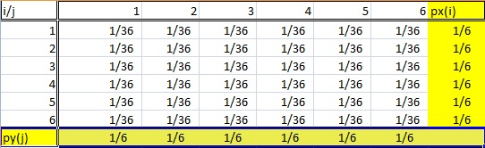
Of course, it’s not quite as simple as that. You can’t just look at any old frequency distribution table and say that the last column (or row) is a “marginal distribution.” Marginal distributions follow a couple of rules:
- The distribution must be from bivariate data. Bivariate is just another way of saying “two variables,” like X and Y. In the table above, the random variables i and j are coming from the roll of two dice.
- A marginal distribution is where you are only interested in one of the random variables . In other words, either X or Y. If you look at the probability table above, the sum probabilities of one variable are listed in the bottom row and the other sum probabilities are listed in the right column. So this table has two marginal distributions.
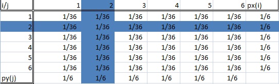
Difference Between Marginal Distribution and Conditional Distribution.
A conditional distribution is where we are only interested in a particular sub-population of our entire data set. In the dice rolling example, this could be “rolling a two” or “rolling a six.” The image below shows two highlighted sub-populations (and therefore, two conditional distributions).
How to Calculate Marginal Distribution Probability
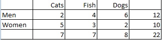
Example question: Calculate the marginal distribution of pet preference among men and women:
Solution:
Step 1: Count the total number of people. In this case the total is given in the right hand column (22 people).
Step 2: Count the number of people who prefer each pet type and then turn the ratio into a probability:
- People who prefer cats: 7/22 = .32
- People who prefer fish: 7/22 = .32
- People who prefer dogs: 8/22 = .36
Tip: You can check your answer by making sure the probabilities all add up to 1.
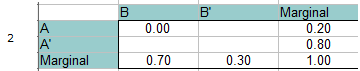
Example question 2 (Mutually Exclusive Events): If P(A) = 0.20, P(b) = 0.70, and both events are mutually exclusive, find P(B’∩A), P(B’∩A’) and P(B∩A’).
If you’re unfamiliar with this notation, P(A’) means “not A”, or the complement. P(B’∩A) means “intersection of not B and A”).
Answer:
You could figure out the probabilities individually, but they’re much easier to figure out using a table.
Step 1: Fill in a frequency table with the given information. The total probability must equal 1, so you can add that to the margins(totals) as well. Simple addition/algebra fills in the marginal blanks. For example, on the bottom row 0.70 + x = 1.00 so The marginal total for B’ must be 0.30.
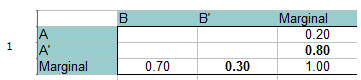
Step 2: Add 0 for the intersection of A and B, at the top left of the table. You can do that because A and B are mutually exclusive and cannot happen together.
Step 3: Fill in the rest of the blanks using simple addition/algebra.
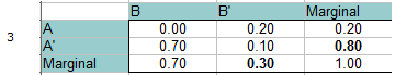
Reading from the table (look at the intersections of the two stated probabilities):
P(B’∩A) = 0.20
P(B’∩A’) = 0.10
P(B∩A’) = 0.70.
Example question 3 (Independent Events): If P(A) = 0.20, P(b) = 0.70, and both events are independent, find P(B’∩A), P(B’∩A’) and P(B∩A’).
Answer: This time, A and B are independent, so the probability of them both happening at the same time is 0.14 (P(A)*P(B) = 0.20 * 0.70 = 0.14). This value goes into the top left (intersection of A and B). Fill out the rest of the table exactly the same way as in the steps above.
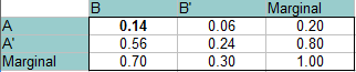
Read the answers from the table (from the intersections of the two probabilities):
- P(B’∩A): 0.06
- P(B’∩A’): 0.24
- P(B∩A’): 0.56.
References
Beyer, W. H. CRC Standard Mathematical Tables, 31st ed. Boca Raton, FL: CRC Press, pp. 536 and 571, 2002.
Agresti A. (1990) Categorical Data Analysis. John Wiley and Sons, New York.
Everitt, B. S.; Skrondal, A. (2010), The Cambridge Dictionary of Statistics, Cambridge University Press.
Lindstrom, D. (2010). Schaum’s Easy Outline of Statistics, Second Edition (Schaum’s Easy Outlines) 2nd Edition. McGraw-Hill Education