Probability Distributions > Kumaraswamy distribution
What is the Kumaraswamy distribution?
The Kumaraswamy distribution was originally proposed by Indian hydrologist Poondi Kumaraswamy in 1980 [1] for variables with lower and upper bounds with a zero-inflation. It is a two-variable family of distributions that is bounded at one and zero. In other words, probabilities outside of the range of 0 to 1 are zero.
It is flexible and can be used to model a variety of shapes, and its probability density function and cumulative distribution function can be written in very simple terms.
Comparison of the Kumaraswamy distribution the Beta Distribution
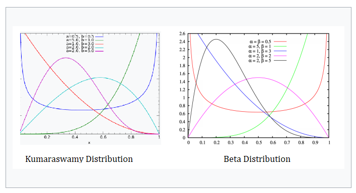
The Kumaraswamy distribution is very similar to the beta distribution and has the same basic shape. So similar in fact, it’s often referred to as a “Beta-like” distribution. However, the Kumaraswamy distribution is simpler to use and in some situations more tractable.
It is often preferred over the Beta in part because the invertible CDF has the closed form:
P(x) = 1 – (1 – xa)b).
Unlike the beta, the Kumaraswamy distribution’s CDF doesn’t contain the incomplete Beta function, which makes it much easier to work with [2].
The PDF and quantile functions also have a closed form, making the Kumaraswamy distribution a more practical choice for many applications—especially simulation studies. Other notable advantages over the beta include explicit formula for moments of order statistics and a simple formula for generation of random variables [3].
Kumaraswamy distribution properties
The probability density function (pdf) for the Kumaraswamy distribution can be expressed, in closed form and without consideration for inflation, as:
![]()
Where a and b are non-negative shape parameters.
The pdf can take on a number of different shapes including bathtub shaped, unimodal, uniantimodal, monotone increasing, and monotone decreasing depending on the values of its parameters. In some cases, singularities exist at the boundaries of the domain. The quantile function is
F-1(p) = 1 – (1- p1/b)1/a
Kumaraswamy’s original work contained bounds at (0, 1). The bounds were extended to include inflations at both extremes [0,1] by S. G . Fletcher in 1996 [4].
References
- Kumaraswamy, P. (1980). “A generalized probability density function for double-bounded random processes”. Journal of Hydrology. 46 (1–2): 79–88. Bibcode:1980JHyd…46…79K. doi:10.1016/0022-1694(80)90036-0. ISSN 0022-1694.
- Michalowicz, J. et al., (2013). Handbook of Differential Entropy. CRC Press.
- Ishaq et al., (2019). On some properties of Generalized Transmuted Kumaraswamy distribution. Pakistan Journal of Statistics and Operation Research; Lahore Vol. 15, Iss. 3, (2019): 577-586.
- Fletcher, S.G.; Ponnambalam, K. (1996). “Estimation of reservoir yield and storage distribution using moments analysis”. Journal of Hydrology. 182 (1–4): 259–275. Bibcode:1996JHyd..182..259F. doi:10.1016/0022-1694(95)02946-x. ISSN 0022-1694