Types of Functions > Cumulative Distribution Function CDF Contents:
What is a Cumulative Distribution Function (CDF)?
The cumulative distribution function (also called the distribution function) gives you the cumulative (additive) probability associated with a function. The CDF can be used to calculate the probability of a given event occurring, and it is often used to analyze the behavior of random variables. More specifically, the CDF of a random variable is the probability that the variable takes a value less than or equal to x. It is one way to describe the distribution of continuous random variables, and can be thought of as an extension of a cumulative frequency table, which measures discrete counts. However, one advantage of the CDF is that it can be defined for every type of random variable, such as discrete, continuous, or mixed. The formula will differ depending on what you are trying to calculate. For example, the CDF for a continuous random variable is represented by the integral: where f(t) represents the density function at point t on the x-axis. It is an extension of a similar concept: a cumulative frequency table, which measures discrete counts. With a table, the frequency is the amount of times a particular number or item happens. The cumulative frequency is the total counts up to a certain number:
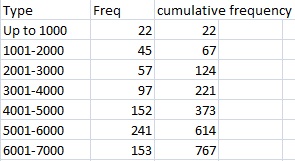
The cumulative distribution function works in the same way, except with probabilities.
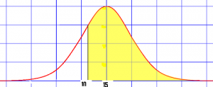
You can use the CDF to figure out probabilities above a certain value, below a certain value, or between two values. For example, if you had a CDF that showed weights of cats, you can use it to figure out:
- The probability of a cat weighing more than 11 pounds.
- The probability of a cat weighing less than 11 pounds.
- The probability of a cat weighing between 11 and 15 pounds.
This means that for any given value of x on the x-axis, F(x) gives us the total area under the curve up to that point on the graph. In other words, it tells us how much “probability mass” has been collected up to that point on the x-axis. In the case of the above scenario, it would be important for, say, a veterinary pharmaceutical company knowing the probability of cats weighing a certain amount in order to produce the right volume of medications that cater to certain weights.
Cumulative Distribution Functions in Statistics
The cumulative distribution function gives the cumulative value from negative infinity up to a random variable X and is defined by the following notation: F(x) = P(X ≤ x). This concept is used extensively in elementary statistics, especially with z-scores. The z-table works from the idea that a score found on the table shows the probability of a random variable falling to the left of the score (some tables also show the area to some z-score to the right of the mean). The normal distribution, the basis of z-scores, is a cumulative distribution function:
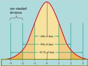
Cumulative distribution functions can be used to analyze data in many different fields such as economics, finance, and engineering. These functions can also be used to calculate expected outcomes and make predictions about future events based on past data points. For example, if you wanted to predict how likely it was for your business to succeed over five years based on market trends from past years, you could use your company’s historical data points and run them through a cumulative distribution function in order to arrive at an answer.
Exceedance distribution function (EDF)
The exceedance distribution tells us how often we can expect rare events.
The exceedance distribution function (EDF) is defined as 1 minus the cumulative distribution function [2]:
EDF = 1 – CDF
The EDF, like the CDF, is bounded between 0 and 1. The CDF tells us what fraction of events are below a specified value. For example, if a measure is at P = 100m with a CDF of 0.4, that tells us 40% of the values are below 100m; the EDF is 1 – 0.4 = 0.6, so 60% of values are above 100m. Because of its complementary nature, the EDF is sometimes called the complementary distribution function.
Heavy tails in an exceedance distribution tell us that there are more occurrences of extreme events; these values represent a lower quantile than a light-tailed distribution [2].
Sometimes the exceedance curve – the graph of a continuous probability exceedance distribution – is called a risk curve or expectation curve. Various formulas have been proposed in the literature.
For example, Sarkadi [3] provided the following formula for the “number of exceedances”,
Where
-
- n and N are independent observations (two sample sizes)
-
- ξ is the number of exceedances, or the number of elements of sample size N which surpass (are larger than) at least n – m + 1 elements of the sample size n( 1 ≤m ≤ n).
Several other authors reference the same formula (e.g., [4]). The formulas have largely become somewhat obsolete with the availability of computer software.
References
- UVA: Image Retrieved April 29, 2021 from: http://www.stat.wvu.edu/srs/modules/normal/normal.html
- Katul, G. Intensity-Duration-Frequency Analysis. Online: https://nicholas.duke.edu/people/faculty/katul/ENV234_Lecture_7.pdf
- Sarkadi, K. (1957). On the Distribution of the Number of Exceedences. The Annals of Mathematical Statistics. Vol 4. P.1021.
- Haight, F. (1958). Index to the Distributions of Mathematical Statistics. National Bureau of Standards Report.