Probability Distributions > Bivariate normal distribution
Contents:
1. Bivariate normal distribution
A bivariate normal distribution is made up of two independent random variables instead of the single one found with the “regular” normal distribution. The two variables in a bivariate normal are both normally distributed and they have a normal distribution when both are added together.
The bivariate normal distribution can be visualized as a surface — a two-dimensional object that can be embedded in three-dimensional space[1]:
Francis Galton (1822-1911) was one of the first mathematicians to study the bivariate normal distribution in depth, during his study on the heights of parents and their adult children. Bravais, Gauss, Laplace, and Plana also studied the distribution in the early nineteenth century [2].
The bivariate distribution can be described in many different ways and as such, there isn’t a unified agreement for a succinct definition. Some of the more common ways to characterize it include:
- Random variables X & Y are bivariate normal if aX + bY has a normal distribution for all a,b ∈ ℝ.
- X and Y are jointly normal if they can be expressed as X = aU + bV, and Y = cU + dV [3]
- If a and b are non-zero constants, aX + bY has a normal distribution [4]
- If X – aY and Y are independent and if Y – bx and X are independent for all a,b (such that ab ≠ 0 or 1), then (X,Y) has a normal distribution [5].
There are dozens of different variants of these definitions. That’s one reason why the bivariate normal is usually defined in terms of its PDF.
PDF of the Bivariate Normal Distribution.
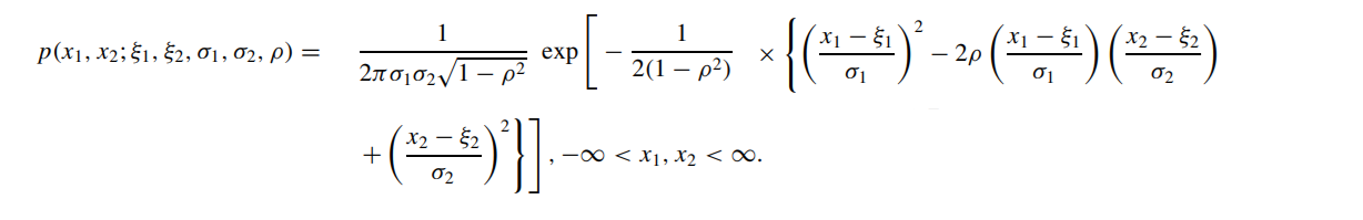
The bivariate normal distribution can be defined as the probability density function (PDF) of two variables X and Y that are linear functions of the same independent normal random variables [6]: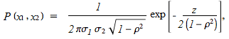
Where:
- μ = mean
- σ = standard deviation
And
![]()
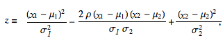
Where:
-
- ρ correlation of x1 and x2.
- V x12= covariance of x1 and x2.
If p = 2, this is equal to the bivariate normal distribution.
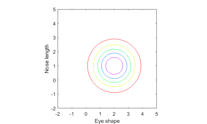
For some excellent gifs that show what happens when a few of these parameters are changed, check out Brad Hartlaub’s page at Kenyon college. This one shows what happens when μ1 is changed: 

2. What is a Multivariate Normal Distribution?
The multivariate normal distribution (also called the multivariate Gaussian distribution) has two or more random variables — so the bivariate normal distribution is a special case of the multivariate normal distribution. That said, while the bivariate normal can be easily visualized (as demonstrated in the gif above), more than two variables poses problems with visualization. Thus, the multinormal can be difficult to wrap your head around — at least, visually. That said, if you’re familiar with matrix algebra it’s fairly easy to work with, and is one of the most important distributions in multivariate statistics.
The multivariate normal distribution is the most important, useful, and widely studied distribution in multivariate statistics because of its:
- Mathematical simplicity: It is relatively easy to work with, so it is easy to obtain multivariate methods.
- Central Limit Theorem (multivariate version): If we have a collection of independent and identically distributed random vectors, then the sample mean vector will be approximately multivariate normally distributed for large samples.
- Applicability to natural phenomena: Many natural phenomena may also be modeled using this distribution, just as in the univariate case [5].
With the bivariate normal distribution, two random variables can be easily visualized — but when more than two are involved, it’s a different story. The multinormal is hard to make sense of without matrix algebra proficiency or some other form of technical savviness – however it still stands as one of the most crucial distributions in understanding today’s multi-dimensional statistics.The bivariate normal distribution (two variables) is easiest to understand because of its notational simplicity; in comparison, distributions with three or more variables require matrix algebra and vector notation.
Multivariate Normal Distribution Properties
The multivariate normal distribution is most often described by its joint density function. A multivariate normal p x 1 random vector X, with population mean vector μ and population variance-covariance matrix σ, will have the following joint density function: ![]()
Where:
- |Σ| = determinant of the variance-covariance matrix Σ
- Σ-1 = inverse of the variance-covariance matrix Σ.
There are several equivalent definitions for the multivariate normal distribution. One way to define it is, given a random vector X = (X1, X2, …, Xd) ∈ ℝd, X is multivariate normal if any linear combination Y = aT X = a1X1 + a2X2 + … + adXd with a ∈ ℝ [6], where T is the transpose of a. Another way to define it is [7]:
For a set of standard normal random variables X = (X1, …, Xk) and Xi, then the expectation E(X) and covariance COV(X) are
E(X) = (0, 0, · · · , 0), COV (X) = I<sub>k</sub>.
Where Ik is the covariance matrix of the random vector X.
Then, for a n dimensional vector µ and n × k matrix A, we have
E(µ + AX) = µ, COV (µ + AX) = AAT
which leads to the following definition:
The distribution of random vector AX is called a multivariate normal distribution with covariance matrix Σ and is denoted by N(0, Σ). And the distribution of µ+AX is called a multivariate normal distribution with mean µ and covariance matrix Σ, N(µ, Σ). Lie Wang.
3. Bravais distribution (another name for bivariate normal distribution)
The Bravais distribution is another name for the bivariate normal distribution, (also sometimes called the bivariate Gaussian or Bivariate Laplace–Gauss distribution).
Teugels & Sundt [7] lists the Bravais distribution as the probability density function of the bivariate normal random vector,
X = (X1, X2)T
which is
Haight [8] refers the reader to a version published in an article in the 1958 Volume 19 of Skandinavisk Aktuarietidskrift. The unnamed author (I was unable to locate a copy of the journal to find the authors name) probably named this distribution after Bravais [9], who developed and published his study of normal frequency distributions in two and more variables.
4. Variance Ratio Distribution (historical name for the bivariate normal distribution)
The “variance ratio distribution” refers to the distribution of the ratio of variances of two samples drawn from a normal bivariate correlated population. Today, we call this the bivariate normal distribution.
The Fisher-Snedicor F Distribution is sometimes called the “Variance Ratio” distribution because it is the distribution of the ratio of two independent variance estimates (S12/S22) [10]. However, this is quite different from the variance ratio distribution in historical literature.
Variance Ratio Distribution History
Haight’s entry in [8] provides the formula:
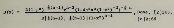
The notation [e]2:65 refers to a 1935 article by Bose [11], titled On the Distribution of the Ratio of Variances of Two Samples Drawn from a Given Normal Bivariate Correlated Population and published in Sankhya, volume 2, 1935. The author, providing a solution to the question of “the distribution function of the ratio of variances obtained from two independent samples,” refers to Fisher’s earlier work [12]
Why the complicated (rarely seen in modern times) formula? The answer is the advent of the computer. Before the computer age (c. 1960s), mathematicians had to refer to tables for the variance ratio distribution F and – sometimes – equations with “great computational difficulty”. In the early days of computers, the distribution also required the “use of excessive amounts of computer time” [13].
Of course, nowadays, we just open our statistics software program and run an algorithm. That’s why you’ll rarely see the actual formula for the variance ratio distribution.
References
- Washington U. Contents / Lesson 20: Pattern Classification Tutorial.
- Balakrishnan,N. & Lai, C. (2009) Continuous Bivariate Distributions.
- Bertsekas & Tsitsiklis (2002). Introduction to Probability (1st ed.).
- Johnson & Kotz. (1972) Distributions in Statistics: Continuous Multivariate Distributions.
- Rao, C. (1975). Some Problems in the Characterization of the Multivariate Normal Distribution.
- Wolfram Mathworld. BND. Retrieved August 4, 2017 from: http://mathworld.wolfram.com/BivariateNormalDistribution.html
- Teugels & Sundt. (2004) Encyclopedia of Actuarial Science. Wiley.
- Haight, F. (1958). Index to the Distributions of Mathematical Statistics. National Bureau of Standards Report.
- Bravais, August, 1846: “Analyse MathCmatique sur les probabilities des erreurs de situation d’un point,” Memoirs Presentes par Divers Savants, 2nd Series, Vol. 9, Institut de France, Acadamie des Sciences, Paris, France, pp. 255-332
- Jolicoeur P. (1999) The distribution of the variance ratio, F = S12/S22. In: Introduction to Biometry. Springer, Boston, MA. https://doi.org/10.1007/978-1-4615-4777-8_9(KENDALL, M. G. The Advanced Theory of Statistics , Volume 1 , London: Charles Griffin and Co., 1945.
- Bose, S., & Mahalanobis, P. C. (1935). On the Distribution of the Ratio of Variances of Two Samples Drawn from a Given Normal Bivariate Correlated Population. Sankhyā: The Indian Journal of Statistics (1933-1960), 2(1), 65–72. http://www.jstor.org/stable/40383720
- Fisher, R. (1924). On a distribution yielding the error function of well known statistics. Proceedings of the International Mathematical Congress, Toronto, 05-813.
- Box, M. & Box, R. (1969). Computation of the variance ratio distribution. Online: https://academic.oup.com/comjnl/article/12/3/277/363429