Contents:
- What is a Binomial Distribution?
- The Bernoulli Distribution
- The Binomial Distribution Formula
- Worked Examples
What is a Binomial Distribution?
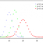
A binomial distribution can be thought of as simply the probability of a SUCCESS or FAILURE outcome in an experiment or survey that is repeated multiple times. The binomial is a type of distribution that has two possible outcomes (the prefix “bi” means two, or twice). For example, a coin toss has only two possible outcomes: heads or tails and taking a test could have two possible outcomes: pass or fail.

- The first variable in the binomial formula, n, stands for the number of times the experiment runs.
- The second variable, p, represents the probability of one specific outcome.
For example, let’s suppose you wanted to know the probability of getting a 1 on a die roll. if you were to roll a die 20 times, the probability of rolling a one on any throw is 1/6. Roll twenty times and you have a binomial distribution of (n=20, p=1/6). SUCCESS would be “roll a one” and FAILURE would be “roll anything else.” If the outcome in question was the probability of the die landing on an even number, the binomial distribution would then become (n=20, p=1/2). That’s because your probability of throwing an even number is one half.
Criteria
Binomial distributions must also meet the following three criteria:
- The number of observations or trials is fixed. In other words, you can only figure out the probability of something happening if you do it a certain number of times. This is common sense—if you toss a coin once, your probability of getting a tails is 50%. If you toss a coin a 20 times, your probability of getting a tails is very, very close to 100%.
- Each observation or trial is independent. In other words, none of your trials have an effect on the probability of the next trial.
- The probability of success (tails, heads, fail or pass) is exactly the same from one trial to another.
Once you know that your distribution is binomial, you can apply the binomial distribution formula to calculate the probability.
Watch the video for an example:
What is a Binomial Distribution? The Bernoulli Distribution.
The binomial distribution is closely related to the Bernoulli distribution. According to Washington State University, “If each Bernoulli trial is independent, then the number of successes in Bernoulli trails has a binomial Distribution. On the other hand, the Bernoulli distribution is the Binomial distribution with n=1.”
A Bernoulli distribution is a set of Bernoulli trials. Each Bernoulli trial has one possible outcome, chosen from S, success, or F, failure. In each trial, the probability of success, P(S) = p, is the same. The probability of failure is just 1 minus the probability of success: P(F) = 1 – p. (Remember that “1” is the total probability of an event occurring…probability is always between zero and 1). Finally, all Bernoulli trials are independent from each other and the probability of success doesn’t change from trial to trial, even if you have information about the other trials’ outcomes.
What is a Binomial Distribution? Real Life Examples
Many instances of binomial distributions can be found in real life. For example, if a new drug is introduced to cure a disease, it either cures the disease (it’s successful) or it doesn’t cure the disease (it’s a failure). If you purchase a lottery ticket, you’re either going to win money, or you aren’t. Basically, anything you can think of that can only be a success or a failure can be represented by a binomial distribution.
The Binomial Distribution Formula

Watch the video for an example:
The binomial distribution formula is:
b(x; n, P) = nCx * Px * (1 – P)n – x
Where:
b = binomial probability
x = total number of “successes” (pass or fail, heads or tails etc.)
P = probability of a success on an individual trial
n = number of trials
Note: The binomial distribution formula can also be written in a slightly different way, because nCx = n! / x!(n – x)! (this binomial distribution formula uses factorials (What is a factorial?). “q” in this formula is just the probability of failure (subtract your probability of success from 1).
![]()
Using the First Binomial Distribution Formula
The binomial distribution formula can calculate the probability of success for binomial distributions. Often you’ll be told to “plug in” the numbers to the formula and calculate. This is easy to say, but not so easy to do—unless you are very careful with order of operations, you won’t get the right answer. If you have a Ti-83 or Ti-89, the calculator can do much of the work for you. If not, here’s how to break down the problem into simple steps so you get the answer right—every time.
Example 1
Q. A coin is tossed 10 times. What is the probability of getting exactly 6 heads?
I’m going to use this formula: b(x; n, P) – nCx * Px * (1 – P)n – x
The number of trials (n) is 10
The odds of success (“tossing a heads”) is 0.5 (So 1-p = 0.5)
x = 6
P(x=6) = 10C6 * 0.5^6 * 0.5^4 = 210 * 0.015625 * 0.0625 = 0.205078125
Tip: You can use the combinations calculator to figure out the value for nCx.
How to Work a Binomial Distribution Formula: Example 2
![]()
80% of people who purchase pet insurance are women. If 9 pet insurance owners are randomly selected, find the probability that exactly 6 are women.
Step 1: Identify ‘n’ from the problem. Using our example question, n (the number of randomly selected items) is 9.
Step 2: Identify ‘X’ from the problem. X (the number you are asked to find the probability for) is 6.
Step 3: Work the first part of the formula. The first part of the formula is
n! / (n – X)! X!
Substitute your variables:
9! / ((9 – 6)! × 6!)
Which equals 84. Set this number aside for a moment.
Step 4: Find p and q. p is the probability of success and q is the probability of failure. We are given p = 80%, or .8. So the probability of failure is 1 – .8 = .2 (20%).
Step 5: Work the second part of the formula.
pX
= .86
= .262144
Set this number aside for a moment.
Step 6: Work the third part of the formula.
q(n – X)
= .2(9-6)
= .23
= .008
Step 7: Multiply your answer from step 3, 5, and 6 together.
84 × .262144 × .008 = 0.176.
Example 3
60% of people who purchase sports cars are men. If 10 sports car owners are randomly selected, find the probability that exactly 7 are men.
Step 1:: Identify ‘n’ and ‘X’ from the problem. Using our sample question, n (the number of randomly selected items—in this case, sports car owners are randomly selected) is 10, and X (the number you are asked to “find the probability” for) is 7.
Step 2: Figure out the first part of the formula, which is:
n! / (n – X)! X!
Substituting the variables:
10! / ((10 – 7)! × 7!)
Which equals 120. Set this number aside for a moment.
Step 3: Find “p” the probability of success and “q” the probability of failure. We are given p = 60%, or .6. therefore, the probability of failure is 1 – .6 = .4 (40%).
Step 4: Work the next part of the formula.
pX
= .67
= .0.0279936
Set this number aside while you work the third part of the formula.
Step 5: Work the third part of the formula.
q(.4 – 7)
= .4(10-7)
= .43
= .0.064
Step 6: Multiply the three answers from steps 2, 4 and 5 together.
120 × 0.0279936 × 0.064 = 0.215.
That’s it!
References
Beyer, W. H. CRC Standard Mathematical Tables, 28th ed. Boca Raton, FL: CRC Press, p. 531, 1987.
Papoulis, A. Probability, Random Variables, and Stochastic Processes, 2nd ed. New York: McGraw-Hill, pp. 102-103, 1984.
Spiegel, M. R. Theory and Problems of Probability and Statistics. New York: McGraw-Hill, pp. 108-109, 1992.
Steinhaus, H. Mathematical Snapshots, 3rd ed. New York: Dover, 1999.
WSU. Retrieved Feb 15, 2016 from: www.stat.washington.edu/peter/341/Hypergeometric%20and%20binomial.pdf