Bivariate Distribution

What is a Bivariate Distribution?

A bivariate distribution (or bivariate probability distribution) is a joint distribution with two variables of interest. The bivariate distribution gives probabilities for simultaneous outcomes of the two random variables.

A discrete joint distribution has at most a countable number of possible outcomes (basically, “countable” means you can label the numbers (like if you’re counting whole numbers 1, 2, 3…).
A continuous joint distribution can be described by a non-negative function [1].

If the two variables are obtained through random sampling, you may be able to find correlations or run a regression analysis to investigate the link between the two variables or to predict future (or past) behavior of those variables. Bivariate distributions are quite common in real life. For example:

In an annual checkup, cholesterol levels and triglyceride levels might be combined to measure heart health.
A gambler might want to know the probability of rolling a six, and then another six.
A café might be interested in studying coffee sales vs. coffee cake sales.
In transportation, the role of alcohol in car crashes is often investigated.

Table Representation of Bivariate Distribution

Unlike many probability distributions, a bivariate distribution doesn’t have a unified look; each distribution is different and it depends on what variables you are studying. A table of rows and columns can be used to display discrete random variables with a finite (fixed) number of values. The rows represent one of the variables, the columns the other. For example, the following table shows the bivariate distribution of tossing a tails if you flip a coin three times: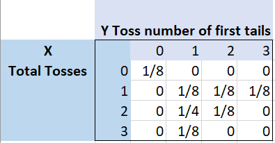

The rows represent the X-values, which in this examples is the total number of tosses.
The columns represent the Y-variable, which is the number of tosses to get the first tails (if no tails occur, this is set to zero).
Each intersection represents an X-Y combination; the probabilities in those cells represent the joint probabilities.

As this is a probability distribution, the probabilities in all the cells add up to 1 [2].

Real Life Uses

Combining two variables in a single distribution, bivariate distributions are quite common both within and outside of the world of mathematics. For example, in medical checkups, cholesterol and triglyceride levels can be combined to assess heart health; gamblers may look at pairing sixes when rolling dice; cafés could try correlating coffee sales with those for cakes; while researchers investigate how alcohol plays into car crashes. Depending on which variables you choose to study however, each bivariate distribution will present unique insights – no unified representation is possible!

Bivariate Normal Distribution

A bivariate normal distribution describes the joint probability distribution of two normally distributed variables (X, Y). Five parameters describe this distribution:

m_x, m_y = mean values of X and Y;
s_x, s_y = standard deviation of X and Y;
r_xy = correlation coefficient between X and Y.

Zero correlation (r = 0) means that X and Y are independent random variables.

Three important characteristics of a bivariate distribution

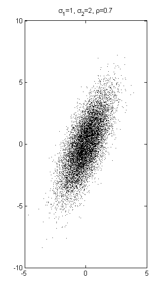
Direction, shape, and strength are three important characteristics of a bivariate distribution. While we can formally define correlation between variables with a correlation coefficient, a scatterplot can give us a rough idea of how much the variables are correlated — or if they bear no relationship at all.

Direction: does the scatterplot trend upwards (a positive linear association), or downwards (a negative linear association)?
Shape: does the scatterplot have a shape of some sort, such as an ellipse? If so, there may be correlation. A random pattern with no discernible shape would indicate no relationship between variables.
Strength: Is the scatterplot long and thin, indicating a strong relationship, or thick and wide, indicating a weak relationship?

This scatterplot is fairly long and thin, indicating a strong relationship [3].

References

Liu, M. STA 611: Introduction to Mathematical Statistics; Lecture 4: Random Variables and Distributions. Retrieved November 10, 2021 from: http://www2.stat.duke.edu/courses/Fall18/sta611.01/Lecture/Lecture04.pdf
Gehrman, J. 6. Bivariate Rand. Vars. Bivariate Probability Distributions. Retrieved November 10, 2021 from: https://www.csus.edu/indiv/j/jgehrman/courses/stat50/bivariate/6bivarrvs.htm
KurtSchwitters, CC BY-SA 3.0 <https://creativecommons.org/licenses/by-sa/3.0>, via Wikimedia Commons