Probability Distributions > Bell-Shaped Distribution
What is a bell shaped distribution?
A bell-shaped distribution is – perhaps not surprisingly – any distribution that looks like the shape of a bell when plotted as a graph. These distributions have one mode (or peak), the mean is close to the median, and the majority of data points cluster close to the distribution’s center.
The normal distribution is the “classic” bell-shaped distribution and is sometimes called the bell-shaped distribution. However, it isn’t the only type of bell-shaped distribution: many other types of probability distributions have a bell curve shape, including the logistic distribution, t-distribution family and the Cauchy distribution. These curves are either narrower than the normal distribution — with more outliers in heavier tails or flatter with fewer outliers in thinner tails.
These distributions have one peak in the center (i.e., they are unimodal distributions) and are symmetric: if you draw a vertical line down the center of the graph, the left half will mirror the right.There are many different bell shaped distributions in statistics. The most well known is “The” bell curve, formally called the normal distribution. However, the normal distribution isn’t the only bell-shaped distribution—there are others, including:
- Hyperbolic Secant Distribution: symmetric member of the exponential family with a mean of 0 and variance of 1. It is similar to the normal distribution both in shape and symmetry but hyperbolic secant has slightly heavier tails [1].
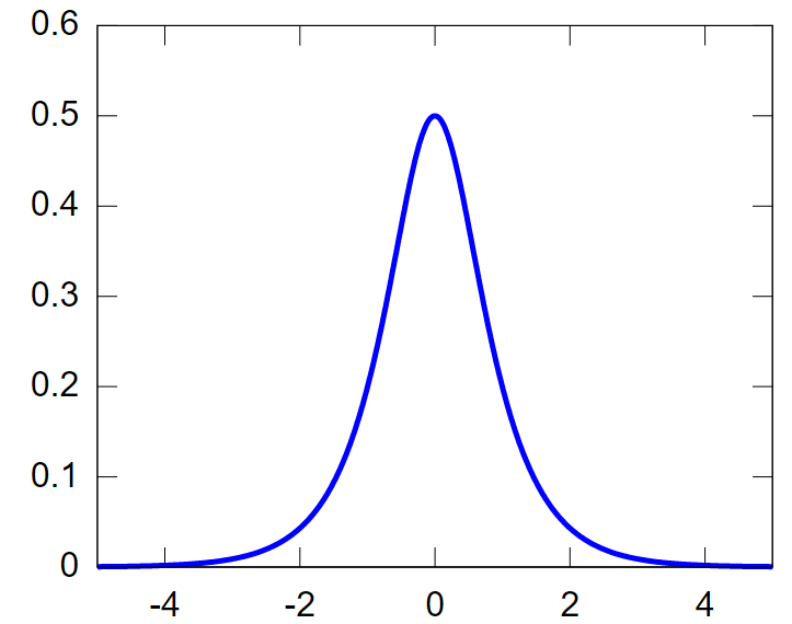
- The logistic distribution also resembles a bell curve; it also has slightly heavier tails than the normal distribution. It appears in logistic regression and feedforward neural networks [2].
- The Cauchy distribution is also bell shaped but the mean and variance are not defined. The median is given by a location parameter θ, and the spread is given by a scale parameter &simga;. The Cauchy distribution occurs as the ratio of two independent standard normal random variables [4].
- A Gaussian mixture model is a probability distribution comprised of several weighted multivariate Gaussian (normal) distributions. The model is an overlapping of bell-shaped curves.
Properties of a Bell Shaped Distribution
A bell shaped distribution is named because it looks like the shape of a bell when plotted on a graph. These distributions share several important properties:
- A single peak in the center (i.e., they are unimodal distributions).
- Symmetry: If you draw a vertical line down the center of the graph, the left half will mirror the right.
Advantages of working with a bell-shaped distribution
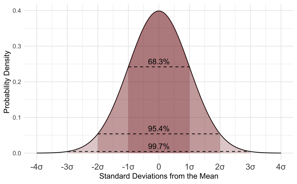
Bell-shaped distributions have many advantages including the fact that their spread is relatively easy to describe with standard deviations — which can be thought of as roughly the average distance data points fall from the mean. Thus, the empirical rule can be used to calculate probabilities.
Other types of distribution shapes
In addition to bell-shaped, we can also describe distributions as skewed, symmetric, or uniform.
- Skewed distribution: is a type of distribution in which one tail is longer than the other. The “bell” is off-center and has a squashed appearance.
- Symmetric distribution: a curve where the left side of the plot mirrors the right side. These do not have to be bell-shaped. They can also be circular or triangular shaped.
- Uniform distribution: A distribution shaped like a rectangle.
References
- M. J. Fischer, Generalized Hyperbolic Secant Distributions, 1 SpringerBriefs in Statistics, DOI: 10.1007/978-3-642-45138-6_1
- Ross, G. Probability/Density Distributions.
- Cunningham, A. Probability Playground: The Cauchy Distribution.
- D Wells, CC BY-SA 4.0, via Wikimedia Commons
- PDF of the logistic distribution. Image: Krishnavedala| Wikimedia Commons