Rayleigh Distribution: Definition, Uses, Mean, Variance

Probability Distributions > Rayleigh distribution

What is the Rayleigh distribution?

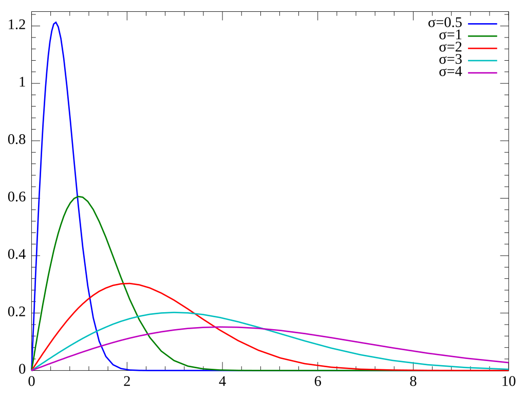
The Rayleigh distribution is a continuous probability distribution for non-negative-valued random variables — variables of 0 or higher. It is skewed right, with its maximum point occurring at a non-zero point. The distribution is used to model the magnitude of random variables that show circular symmetry.

The distribution is named after William Strutt, Lord Rayleigh, a British mathematician and physicist who first studied it in the context of the distribution of sound intensity. 

Rayleigh distribution properties

The notation X Rayleigh(σ) means that the random variable X has a Rayleigh distribution with shape parameter σ.

The probability density function (pdf) (X > 0) is:
Where

• e = Euler’s number.
• (σ) = shape parameter 

When a Rayleigh is set with a shape parameter (σ) of 1, it is equal to a chi square distribution with 2 degrees of freedom. As the shape parameter increases, the distribution gets wider and flatter.

 

The characteristic function is:

φ(t) = 1 – √(π/2) * σt * exp(-σ^2t2/2) * Ei(σ^2t2/2)

where Ei(x) is the exponential integral function.

The moment generating function is:

M(t) = 1 + √(π/2) * σt * exp(-σ^2t2/2) * Erf(σt/√(2)),

where Erf(x) is the error function. 

Other properties:

• Mean = σ√(π/2).
• Variance = σ²((4 – π)/2).
• Mode = σ * √(ln(4)).
• Skewness = 2/√(ln(4)),
• Kurtosis = 6 + ln(4).

The expected value of a Rayleigh is also the same as the mean: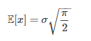
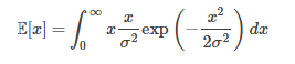
How this equation is derived involves solving an integral, using calculus:

• The expected value of a probability distribution is: E(x) = ∫ xf(x)dx.
• Substituting in the Rayleigh probability density function, this becomes the improper integral: Where:
  • exp is the exponential function,
  • dx is the differential operator.

• Solving the integral for you gives the Rayleigh expected value of σ √(π/2)

The variance is derived in a similar way, giving the variance formula of: Var(x) = σ²((4 – π)/2).

Real life applications of the Rayleigh Distribution

The Rayleigh has many applications in real-world situations. For example, it can be used to model data that is distributed across multiple categories, such as the size of particles in a sample or the intensity of light at different wavelengths. It can also be used to model data that varies over time, such as the arrival rate of customers at a store or the amount of time it takes for an event to occur.

Some specific real-world examples:

• Signal Processing: This distribution can model the magnitude of noise in signals, as noise — like the Rayleigh distribution — often shows circular symmetry.
• In telecommunications, the Rayleigh can model radio signal fading, a process where signal strength diminishes due to interference from other signals or obstacles. It can estimate the likelihood of a radio signal fading below a particular level.
• In oceanography, the height of ocean waves can be modeled using the Rayleigh distribution. Ocean waves are typically depicted as random variables with circular symmetry, and the Rayleigh distribution can estimate the probability an ocean wave will reach beyond a certain height.
• Engineering: In engineering, the Rayleigh can model material strength, which is often depicted as a random variable with circular symmetry. Using the Rayleigh distribution, one can estimate the likelihood of a material failing under a specific load.

In addition, the Rayleigh can be used to estimate unknown parameters in other distributions, such as the normal (Gaussian) distribution. Estimating unknown parameters is important in statistics because it allows us to make predictions about future events. For example, we can estimate unknown parameters in a distribution by fitting a Rayleigh distribution to it and estimating the scale and shape parameters; if we know that — for example — the mean and variance of a dataset equal to 5, we can use this information to predict that 95% of all future values will fall between 0 and 10 (using the empirical rule).

Related distributions

The Rayleigh distribution is a special case of the Weibull distribution with a scale parameter of 2. When a Rayleigh is set with a shape parameter (σ) of 1, it is equal to a chi square distribution with two degrees of freedom.

The Gompertz-Rayleigh distribution is an extension of the Rayleigh distribution that allows for better modeling of highly-skewed (off-center) datasets compared to compound distributions [1]. A similarly named but unrelated distribution is a generalized Gompertz-Rayleigh distribution, proposed by Bradley [2] as a potential survival distribution for modeling risk.

Many other generalized forms have been proposed including Kundu & Raqab’s ‘s generalized Rayleigh [3], Merovci & Eltabal’s Weibull-Rayleigh [4], and Ahmad et al.’s transmuted Rayleigh distribution [5], but Mohammed et. al [6] proposed adding the Gompertz-G family of distributions to have more flexibility and greater skew.

The Gompertz-G family of distributions was introduced by Mohammed et al. in a manner similar to others recently developed. The mathematical properties of the new family are available from a linear mixture of exponentiated-G densities and the creators claim two main advantages in these recent methods:

• They create distributions with several known particular cases.
• The added parameters may provide better fits of the generated distributions to data sets and they can have physical interpretations.

History of the Rayleigh distribution

The Rayleigh distribution was initially studied by Lord Rayleigh (John William Strutt) in 1880. Rayleigh, a British mathematician, is known for his work on wave theory and the discovery of the scattering phenomenon named after him — Rayleigh scattering.

In his paper “On the Problem of the Distribution of Energy in a Beam of Light“, Rayleigh demonstrated that the distribution of sound intensity in a light beam can be represented by a continuous probability distribution, now known as the Rayleigh distribution.

Since then, the Rayleigh distribution has been applied in various fields, such as signal processing, telecommunications, oceanography, engineering, and statistics.

References

1. Mohammed, F. et al. (2020). A study of some properties and goodness-of-fit of a Gompertz-Rayleigh model. Asian journal of probability and statistics, Page 18-31.
2. Bradley, D. et al. (1984). A generalized Gompertz-Rayleigh model as a survival distribution. Mathematical Biosciences Volume 70, Issue 2, August 1984, Pages 195-202
3. Kundu, D. & Raqab, M. Generalized Rayleigh Distribution: Different methods of estimations. Comp. Stat. & Data Anal. 2005; 49:187-200
4. Merovci, F & Eltabal, I. Weibull-Rayleigh distribution: Theory and applications. Appl. Math & Inf. Sci. 2015; 9(5): 1-11.
5. Ahmad et al. Transmuted inverse Rayleigh distribution: A generalization of the inverse Rayleigh distribution. Math Theo. & Mod. 2015; 4(7):90-98.
6. Mohamed et. al. Gompertz-G family of distributions. November 2016Journal of Statistical Theory and Practice. 11(1)https://www.researchgate.net/publication/311105965_The_Gompertz-G_family_of_distributions