Probability Distributions > Laplace Distribution
What is a Laplace Distribution?
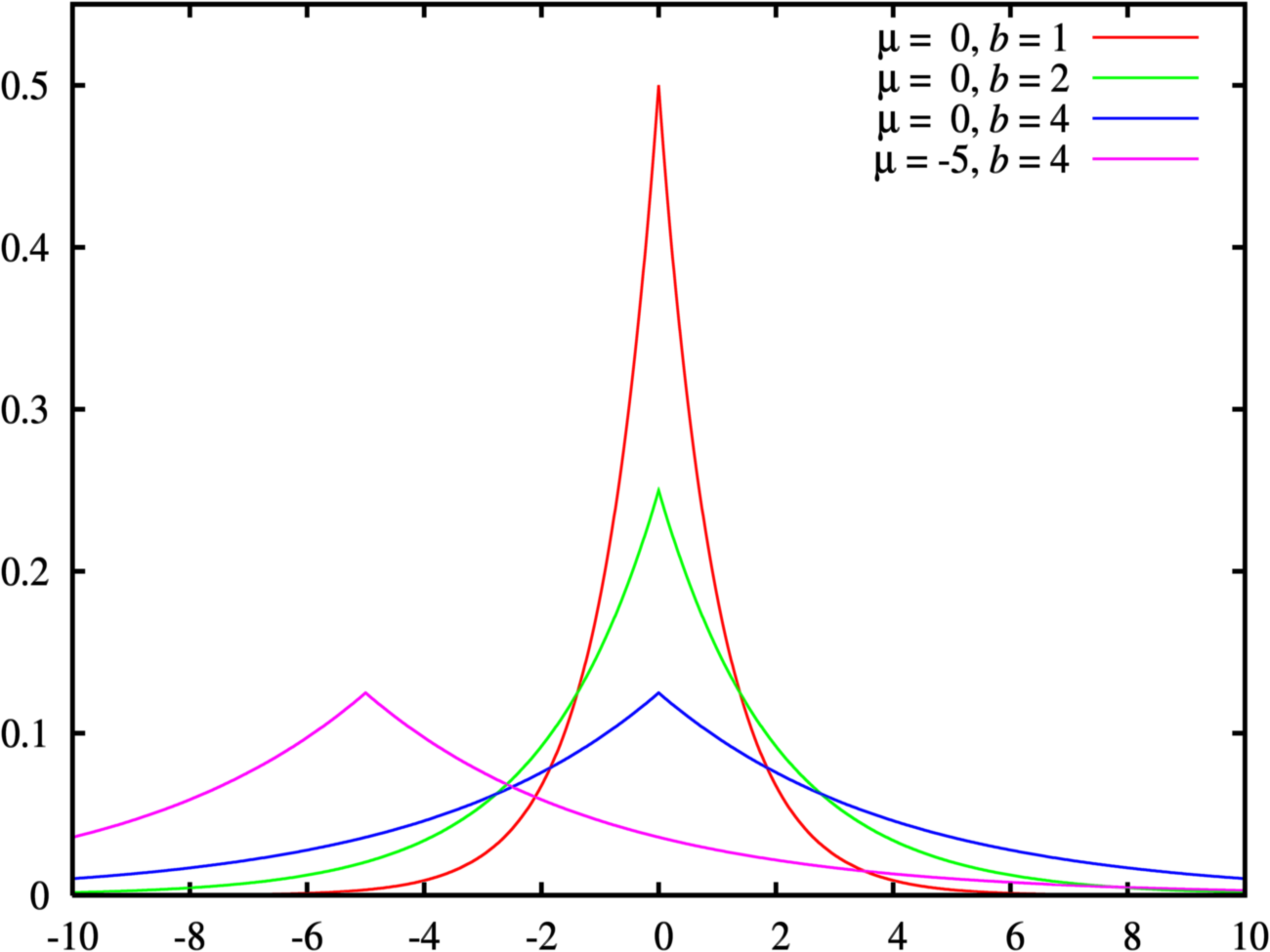
The Laplace distribution, one of the earliest known probability distributions, is a continuous probability distribution named after the French mathematician Pierre-Simon Laplace. Like the normal distribution, this distribution is unimodal (one peak) and it is also a symmetrical distribution. However, it has a sharper peak than the normal distribution.
The Laplace distribution is the distribution of the difference of two independent random variables with identical exponential distributions (Leemis, n.d.). It is often used to model phenomena with heavy tails or when data has a higher peak than the normal distribution.
This distribution is the result of two exponential distributions, one positive and one negative; It is sometimes called the double exponential distribution, because it looks like two exponential distributions spliced together back-to-back.
The general formula for the probability density function (PDF) is:
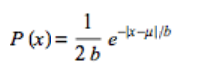
where:
- μ (any real number) is the location parameter and
- β (must be > 0) is the scale parameter; this is sometimes called the diversity.
Scale and Location Parameters
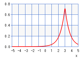
The shape of the Laplace distribution is defined by the location parameter and scale parameter. The following image was created with this online Casio calculator (μ = 3, β = 0.7), which enables you to create various PDFs and CDFs for the distribution.
Mean, Variance, Skewness, Kurtosis
(Härdle & Simar, 2015)
Classical Univariate Laplace
The Laplace distribution with a location parameter of zero (i.e. a mean of zero) and scale parameter of one (i.e. variance σ2 of one) is called the classical univariate Laplace distribution. The function for this particular version of the distribution is:
f(x) = e-|x| / 2.
Where e-x is the exponential function.
CDF
The cumulative distribution function (CDF) of the Laplace distribution is found with calculus; it is the integral of the PDF. You can think of an integral as the area under the curve. It’s the same idea as finding the area under a curve to find probabilities in normal distributions.
The formula for the CDF is:
![]()
Where sgn is the sign function.
For more information on solving integrals, see:
- Definite Integrals (CalculusHowTo.com)
- Accumulation Function (CalculusHowTo.com)
Software
Despite being one of the oldest probability distributions, it isn’t commonly used. Therefore, it can be a challenge to find functions for this distribution on popular software, like Excel. However, many statistical software packages do offer options, including Maple and SPSS.
Check out our YouTube channel for hundreds of statistics help videos.
References
Härdle, W. & Simar, L. (2015). Applied Multivariate Statistical Analysis. Springer.
Leemis, L. (n.d.). Exponential / Laplace. Retrieved January 10, 2018 from: http://www.math.wm.edu/~leemis/chart/UDR/PDFs/ExponentialLaplace.pdf
Weisstein, Eric W. “Laplace Distribution.” From MathWorld—A Wolfram Web Resource. http://mathworld.wolfram.com/LaplaceDistribution.html