Probability Distributions > Contents:
See also: Superfactorial: Definition (Sloane, Pickover’s)
What is a Factorial?
Factorials (!) are products of every whole number from 1 to n. In other words, take the number and multiply through to 1. For example:
- If n is 3, then 3! is 3 x 2 x 1 = 6.
- If n is 5, then 5! is 5 x 4 x 3 x 2 x 1 = 120.
It’s a shorthand way of writing numbers. For example, instead of writing 479001600, you could write 12! instead (which is 12 x 11 x 10 x 9 x 8 x 7 x 6 x 5 x 4 x 3 x 2 x 1).
What is a factorial used for in stats?
In algebra, you probably encountered ugly-looking factorials like (x – 10!)/(x + 9!). Don’t worry; You won’t be seeing any of these in your beginning stats class. Phew! The only time you’ll see them is for permutation and combination problems. The equations look like this: 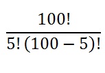
And that’s something you can input into your calculator (or Google!).
Factorial Distribution
The factorial distribution is a distribution for which successive frequencies are factorial qualities. It can also be defined as a distribution that happens when variables are independent events.
1. The factorial distribution as factorial qualities
Irwin [1] defines the factorial distribution (also called the inverse factorial series distribution) as a distribution that occurs when successive frequencies are factorial qualities, with the form
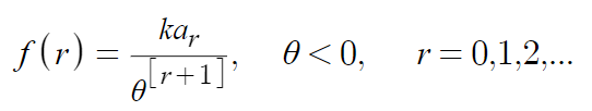
where x[0] = 1, x[r] = x(x + 1) … (x + r – 1) denotes the ascending factorial (note: x does not appear in the general factorial distribution distribution, because it can be used to model any factorial distribution, regardless of the value of x).
A special case is Waring’s distribution, with ar = a[r] / θ[r + 1]. In addition, if a = 1 and θ – a = p, the factorial distribution becomes the Yule distribution [3].
2. A factorial distribution as independent events
A factorial distribution is one of the simplest probability distributions, because the variables don’t interact at all. It can be used to determine the probability of multiple events occurring at once or consecutively, and it can be written in many different ways.
This type of distribution happens when a set of variables are independent events. This means that the variables don’t interact at all; given two events x and y, the probability of x doesn’t change when you factor in y. For example, if event x is a coin toss and event y is choosing a card from a deck, those events don’t interact and so are independent.
Therefore, the probability of x given that y has happened, P(x | y), will be the same as the probability of x, written as p(x). This type of distribution allows us to calculate probability based on certain factors without having to consider other variables or factors.
The factorial distribution can be written in many ways [4, 5]:
- p(x, y) = p(x) p(y)
- p(x, y ,z) = p(x) p(y) p(z)
- p(x1, x2, x3, x4) = p(x1) p(x2) p(x3) p(x4)
- P(x) = ΣP(x | y) * P(y)
Note that none of these terms include a factorial (!) symbol; that’s because the factorial distribution doesn’t contain any factorials per se; it is named because successive frequencies are factorial quantities. Factorials (!) are products of whole numbers up to the number of interest. For example, 3! (read “three factorial”) equals 3 * 2 * 1 = 6.
The equation P(x) = ΣP(x | y) * P(y) states that the total probability of event x happening is equal to the sum of all probabilities for each separate event multiplied together. For example, if you want to find out the probability that two people out of five will get sick from eating contaminated food, you would use this equation to determine your answer. The total probability would be 0.25 because each individual has a 0.5 chance of getting sick (assuming everyone has an equal chance).
A more general way of writing the factorial distribution for three or more variables is [6]
P(x1, x2, … ,xn) = P(x1) · P(x2 · …· P(xn) = P(x1, x2, … xn)= Πi P(xi).
The Π (uppercase pi) symbol is the product operator, which is used for multiplication in the same way that the uppercase sigma (Σ) symbol is used for summation.
Factorial Distribution Examples
We like to work with factorial distributions because their statistics are easy to compute. In some fields such as neurology, situations best represented by complicated, intractable probability distributions are approximated by factorial distributions in order to take advantage of this ease of manipulation. One example of an often-encountered factorial distribution is the p-generalized normal distribution, represented by the equation 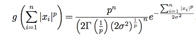 When p = 2, this is the normal distribution.
Calculating a factorial distribution requires some basic knowledge of statistics and probability theory. You need to understand how independent events interact with one another and how they affect each other’s probabilities. Once you have these concepts down, you can use them to calculate any number of scenarios involving independent events. To do so:
- Start by writing out the separate probabilities for each individual event (P(x) and P(y)).
- Then multiply those numbers together and add them up: Σ P (x |y) * P(y).
- Finally, divide your result by 1 minus whatever number results from subtracting your original probabilities (1- [P(x)-P(y)]). This will give you your final answer—the likelihood that both events will occur simultaneously or sequentially.
Application example: wake-sleep algorithm
One application is in the wake-sleep algorithm in machine learning (a stack of layers that represents data); the probability of a whole vector is the product of its individual terms [5]. For example, lets say that you have three probabilities of hidden units in a layer:
0.3; 0.6; 0.8.
The probability that these units have a state 1, 1, 1 if the distribution is factorial is
p(1, 1, 1) = 0.3 * 0.6 * 0.8
Similarly, The probability that these units have a state 1, 0, 1 is
p(1, 0, 1) = 0.3 * (1 – 0.6) * 0.8.
Gamma Function
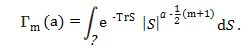
The Gamma function (sometimes called the Euler Gamma function) is related to factorials by the following formula: Γ(n) = (x – 1)!. In other words, the gamma function is equal to the factorial function. However, while the factorial function is only defined for non-negative integers, the gamma can handle fractions as well as complex numbers. The multivariate gamma function (MGF) is an extension of the gamma function for multiple variables. While the gamma function can only handle one input (“x”), the multivariate version can handle many. It is usually defined as:
References
- Irwin, J. (1963). The place of mathematics and biological statistics. Journal of the Royal Statistical Society. Series A, 126, 1-45.
- Olshausen, B. (2004). A Probability Primer. Retrieved December 27, 2017 from: Retrieved from http://redwood.berkeley.edu/bruno/npb163/probability.pdf