< List of probability distributions > Gig Distribution
The term GIG distribution usually refers to the generalized inverse Gaussian distribution (e.g. Zhang et al [1], Pothula [2]). However, the term is sometimes used to mean the generalized integer gamma distribution instead (e.g., Coelho [3]).
Contents:
1.Generalized Inverse Gaussian Distribution (GIG distribution)
The Generalized Inverse Gaussian Distribution (GIG), denoted GIG(λ, ψ, χ), is a common distribution used in several areas of statistics, including finance, geostatistics, and statistical linguistics. The GIG model is a popular distribution in probability theory for continuous probability distributions due to its versatility and applicability in different areas of study.
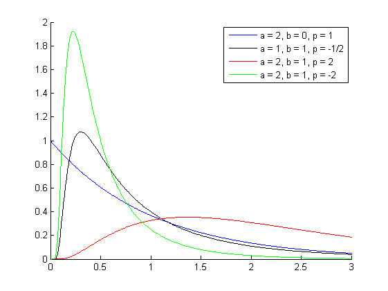
The GIG distribution is able to produce symmetric as well as asymmetric distributions. It can also yield a distribution model that approaches a normal/Gaussian or even a Laplace distribution. While the GIG is typically used in continuous data sets, being able to model such a broad range of distributions makes the GIG very versatile.
The distribution does not have a closed for for its cumulative distribution function (CDF).
The probability density function (PDF) can be expressed with Bessel functions as [4]
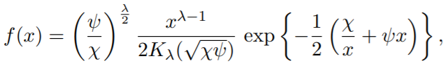
where x > 0 and Kλ is the modified Bessel function.
Parameters must satisfy tthree requirements:
- χ > 0, ψ ≥ 0, when λ < 0,
- χ > 0, ψ > 0, when λ = 0,
- χ ≥ 0, ψ > 0, when λ > 0.
Special cases of the GIG distribution include the inverse normal/Gaussian distribution (for λ = −1/2) and gamma distribution ( for ψ = 0) [5].
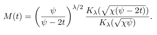
The moment generating function is
The name generalized inverse Gaussian distribution originates with Ole Barndorff-Nielsen, who came across the largely underdeveloped distribution while studying hyperbolic distributions. Barndorff-Nielsen et al. [6] proved that any GIG distribution with a non-positive power parameter is the distribution of the first hitting time to level 0 for a time-homogeneous diffusion process with state space [0,∞). This suggests that the GIG distribution could be useful as a lifetime distribution or the time distribution between successive events in a renewal process [7].
Although Barndorff-Nielsen popularized the GIG distribution, it was Étienne Halphen who first discovered the GIG distribution in 1941 (albeit under a different name). Its properties are discussed in Bent Jørgensen’s Lecture Notes in Statistics [8].
Applications
The GIG distribution has multiple applications in many industries. One common application is in the pricing of options in finance. Options are complex financial instruments used to hedge against stock price volatility. Options pricing models that incorporate the GIG distribution are preferred due to their ability to handle skewness and kurtosis more efficiently than standard models.
Another application of the GIG distribution is its use in spatial statistics, particularly in the study of geostatistics. Geo-statistics is used to analyze and understand geographically dependent data that has a spatial correlation. By using the GIG distribution, we can model the data more accurately, incorporating skewness, and heavy tails in predictions.
Statistical linguistics is a rapidly growing field, and it also benefits from the use of the GIG distribution. In statistical linguistics, texts are analyzed to understand the underlying language structure best. In addition, model inference can be used to generate texts that are grammatically correct and stylistically similar to the input corpus. The GIG distribution is helpful in these cases, as it can generate syntactically valid texts within the style of the original input.
2. Generalized integer gamma distribution
The generalized integer gamma distribution (also called the GIG distribution) is a special case of the generalized chi-squared distribution and involves the distribution of the sum of independent gamma distributed random variables with distinct rate parameters and integer shape parameters. It is also called the discrete gamma distribution or the integer gamma distribution.
A common form of the probability density function (PDF) of the generalized integer gamma distribution is
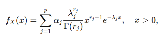
Where
- p = depth (number of component gamma distributions)
- rj = integer shape parameters of each gamma component
- λj = rate parameters of each gamma component.
To find the coefficients, αj, the moments are typically matched. Equivalently, you can solve a system of linear equations derived from the convolution structure.
The integer shape parameter affects the distribution’s probability mass function (PMF), which only takes integer values.
The distribution is a special case of the chi-squared distribution where random variables follow a gamma distribution.
Properties of the GIG distribution include:
- Mean value = integer shape parameter / rate parameter,
- Variance = integer shape parameter / square of the rate parameter,
- Mode = floor(x), where the variable x is the sum of the gamma-distributed random variables.
If the Generalized Integer Gamma distribution is represented as a mixture of gamma distributions with integer shape parameters, its cumulative distribution function (CDF) can be expressed as a linear combination of the CDFs of those component gamma distributions: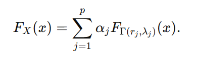
If you know the mixture weights αj, the shape parameters rj, and the rate parameters λj, you can calculate the CDF as a weighted sum of the incomplete gamma function ratios: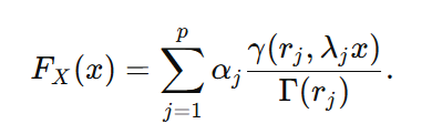
Although the GIG distribution isn’t very common, it does have some specific applications in queuing theory, probability theory, and discrete data analysis. It is relevant when data points are discrete and the underlying probability distribution is unknown. In actuarial science, the distribution can model the number of claims an insurance company receives in a specific time period.
There isn’t a closed form expression for the probability mass function (PMF) of the sum of gamma-distributed variables. Because we can’t use a neat probability formula, the distribution parametrization must be well defined. In other words, you must be sure about which shape and scale parameters you use. Also, organize your data well because the parameters you find aren’t unique; they aren’t tied to one specific arrangement of variables.
References
- Zhang et. al. EP-GIG Priors and Applications in Bayesian Sparse Learning Journal of Machine Learning Research 13 (2012) 2031-2061 Submitted 9/11; Revised 2/12; Published 6/12
- Pothula, P. Random Variate Generation from Generalized Inverse Gaussian Distribution. Thesis. Retrieved April 20, 2023 from: https://scholarworks.unr.edu/bitstream/handle/11714/4019/Pothula_unr_0139M_10896.pdf?sequence=1&isAllowed=y
- Coelho, C. A mixture of Generalized Integer Gamma distributions as the exact distribution of the product of an odd number of independent Beta random variables: applications. Journal of Interdisciplinary Mathematics Vol. 9 (2006), No. 2, pp. 229–248. Taru Publications
- R-forge distributions Core Team Handbook on probability distributions University Year 2009-2010
- Johnson, Norman L.; Kotz, Samuel; Balakrishnan, N. (1994), Continuous univariate distributions. Vol. 1, Wiley Series in Probability and Mathematical Statistics: Applied Probability and Statistics (2nd ed.), New York: John Wiley & Sons, pp. 284–285, ISBN 978-0-471-58495-7, MR 1299979
- Barndorff-Nielsen O., Blsild P., Halgreen C. First hitting time models for the generalized inverse Gaussian distribution Stochastic Process. Appl., 7 (1) (1978), pp. 49-54
- Mimi Zhang, Matthew Revie, John Quigley, Saddlepoint approximation for the generalized inverse Gaussian Lévy process, Journal of Computational and Applied Mathematics, Volume 411, 2022.
- Jørgensen, B. (2012). Statistical Properties of the Generalized Inverse Gaussian Distribution. Lecture notes in statistics. Springer Science & Business Media.