Probability Distributions > Weibull Distribution and Analysis
Contents:
What is the Weibull Distribution?
The Weibull distribution is a continuous probability distribution named after Swedish mathematician Waloddi Weibull. He originally proposed the distribution as a model for material breaking strength, but recognized the potential of the distribution in his 1951 paper A Statistical Distribution Function of Wide Applicability. Today, it’s commonly used to assess product reliability, analyze life data and model failure times. The Weibull can also fit a wide range of data from many other fields, including: biology, economics, engineering sciences, and hydrology (Rinne, 2008).
Although it’s extremely useful in most cases, the Weibull isn’t an appropriate model for every situation. For example, chemical reactions and corrosion failures are usually modeled with the lognormal distribution.
Weibull Distribution PDFs
Two versions of the Weibull probability density function (pdf) are in common use: the two parameter pdf and the three parameter pdf. Different authors use different notation, which makes the notation a little confusing if you’re looking at different texts. For example, The Engineering Statistics Handbook uses gamma(γ) to represent the shape parameter, while other authors (e.g. Fritz Scholz, writing for Boeing) use beta (β). I’ve included the different notations I have found in the pdf information below. If you find more, please don’t hesitate to let me know by leaving a comment on our Facebook page.
For clarity, I’m staying with the same notation for all formulas: γ for the shape parameter, x as the variable, and μ for the location parameter.
Three parameter Weibull
The formula for the probability density function of the three parameter general Weibull distribution is:
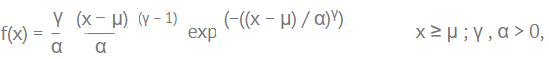
Where:
- γ is the shape parameter (also known as the Weibull slope or the threshold parameter). Note: some authors use β, m, or k.
- α is the scale parameter, also called the characteristic life parameter. Note: some authors use c, ν or η instead. I found a single text (Glantz & Kissell, 2013) using γ.
- μ is the location parameter, also called the waiting time parameter or sometimes the shift parameter. Note: μ the time to failure, is not included in the two parameter version.
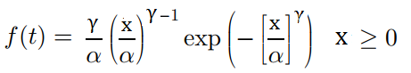
When μ = 0 and α = 1, the formula for the pdf reduces to:
![]()
which is the standard Weibull distribution.
Two parameter Weibull
The formula is practically identical to the three parameter Weibull, except that μ isn’t included:
The two parameter Weibull is often used in failure analysis, because no failure can happen before time zero. If you know μ, the time when the failure happens, you can subtract it from x (i.e. time t). Therefore, when you move from the two-parameter to the three-parameter version, all you have to do is replace each instance of x with (x – μ).
Gamma and Failure Rates
The value for the shape parameter (γ) determines the failure rates:
- If gamma is less than 1, then the failure rate decreases with time (i.e. the process has a large number of infantile or early-life failures and fewer failures as time passes).
- For γ = 1: the failure rate is constant, which means it’s indicative of useful life or random failures.
- If γ > 1: the failure rate increases with time (i.e. the distribution models wear-out failures, which tend to happen after some time has passed).
EVD Type III
Under some specific parameters, the Wiebull is an example of an extreme value distribution (EVD) and is sometimes called EVD Type III. Extreme values are data points that are either very high, or very low, relative to the other points in the set; These values are found in a distribution’s tails. EVDs are the limiting distributions for these values. The other two EVDs are the Gumbel distribution (EVD Type I) and the Fréchet distribution (EVD Type II).
The Weibull Family
The Weibull distribution is a family of distributions that can take on many shapes, depending on what parameters you choose.
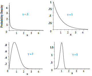
The Weibull distributions above include two exponential distributions (top row), a right-skewed distribution (bottom left) and a symmetric distribution (bottom right). The exponential distribution is a special case of the Weibull distribution, which happens when the Weibull shape parameter equals 1.

Changing α, the scale parameter, does not change the type of shape, but it does stretch out the existing shape. If the other two parameters are kept the same:
- Increasing α results in the graph being stretched to the right. The height will decrease.
- Decreasing α results in the graph being shrunk to the left (towards zero). The height will increase.
Weibull Analysis
Weibull analysis involves using the Weibull distribution (and sometimes, the lognormal) to study life data analysis — the analysis of time to failure. For example, Weibull analysis can be used to study:
- Lifetimes of medical and dental implants,
- Components produced in a factory (like bearings, capacitors, or dialetrics),
- Warranty analysis,
- Utility services,
- Other areas where time-to-failure is important.
The analysis isn’t limited to production; it is applicable to the design stage and in-service time as well.
In the past, the techniques to perform Weibull analysis by hand were tedious and lengthy. The process has now been replaced by statistical software programs and is today the most widely used technique for analyzing lifetimes data in the world.
The major advantages to using Weibull analysis is that it can be used for analyzing lifetimes with very small samples. It also produces an easy-to-understand plot.
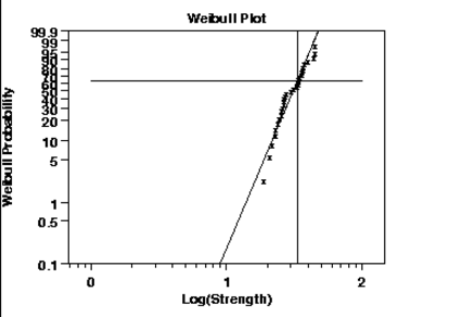
The horizontal axis on a Weibull plot shows lifetimes or aging parameters like mileage, operating times, or cycles of use. The vertical axis shows cumulative (additive total) percentage failures.
The analysis includes:
- Forecasting when spare parts will be needed.
- Implementing a plan for corrective action.
- Planning maintenance and cost effective replacement strategies.
- Plotting and interpreting data.
- Predicting failures.
References
Engineering Statistics Handbook (n.d.). Retrieved October 25, 2017 from: http://www.itl.nist.gov/div898/handbook/apr/section1/apr162.htm
ETH Zurich Department of Mathematics. (n.d). The R Stats Package.
Johnson, N. L., Kotz, S. and Balakrishnan, N. (1995) Continuous Univariate Distributions, volume 1, chapter 21. Wiley, New York.
Glantz & Kissell (2013). Multi-Asset Risk Modeling: Techniques for a Global Economy in an Electronic and Algorithmic Trading Era. Academic Press.
Rinne, H., (2008). The Weibull Distribution: A Handbook. CRC Press.
Scholz, F. (1999). Weibull reliability analysis. Boeing Phantom Works. Retrieved October 25, 2017 from: https://www.researchgate.net/file.PostFileLoader.html?id=54d7377bd2fd643a488b459f&assetKey=AS%3A273694931259401%401442265364239
Weibull, W., (1951). A Statistical Distribution Function of Wide Applicability, Journal of Applied Mechanics.