Probability Distributions > Gompertz-Makeham distribution
What is the Gompertz-Makeham Distribution?
The Gompertz-Makeham distribution, sometimes called the Makeham distribution, is a generalization of the Gompertz distribution. This continuous probability distribution is a popular model for adult lifetimes, especially in insurance as it can be used to estimate the probability that a person will die within a certain age range.
In 1825, Benjamin Gompertz theorized that the probability of dying increases exponentially with age — a law now called the Gompertz law of mortality. Gompertz’s law was refined by William Makeham in 1860 to include an age-independent component, such as accidents, infections, and other external causes of death. This law became known as the Makeham law of mortality. Gompertz’s hypothesis that the probability of dying increases in geometrical progression marked an “epoch in the history of actuarial science” [1].
Together, the Gompertz and Makeham laws of mortality form the basis for the Gompertz-Makeham distribution, which uses a combination of exponential and power functions to model the probability density function (pdf) of lifetimes.
Gompertz-Makeham distribution properties
The probability density function is:
![]()
Where
- α is the Gompertz rate parameter, which controls the shape of the curve and represents the rate at which mortality increases with age.
- β is the Makeham rate parameter, which represents the age-independent component of mortality.
- γ is the scale parameter, which sets the overall scale of the distribution.
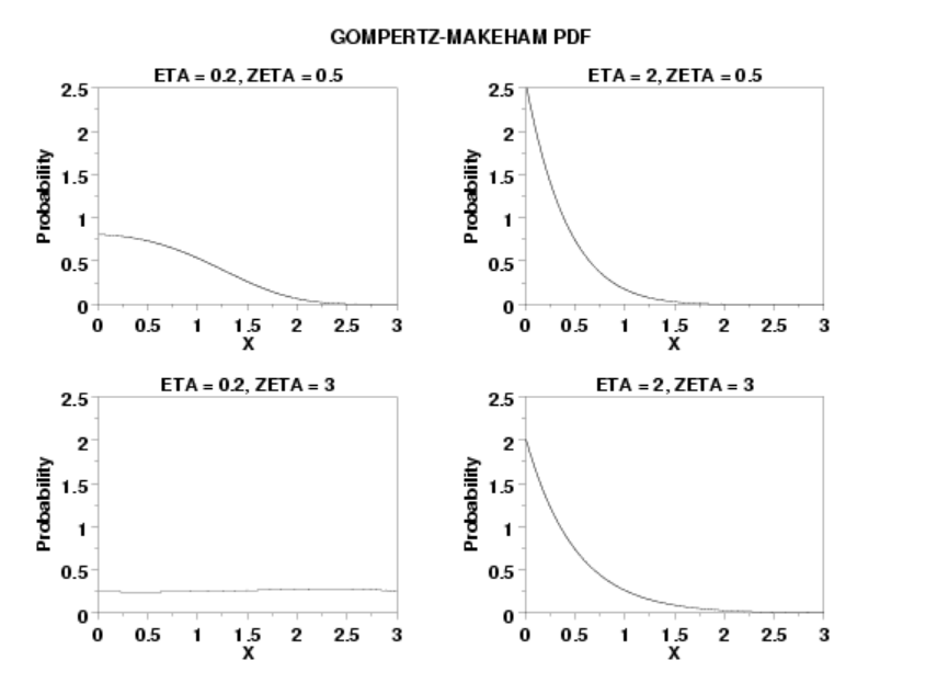
The distribution is defined over the interval [0, ∞] and can take on a wide variety of shapes: The PDF may be unimodal, or in some cases monotonically decreasing with a singularity as x approaches zero. The distribution can also be fat tailed (decreases algebraically) or thin tailed (decreases exponentially), depending on the parameters [2]:
- γ = shape parameter.
- δ = frailty parameter.
Note that “frailty” here doesn’t refer to individuals, but rather populations. More specifically, it is an unobservable univariate statistical variable Z that describes a relationship with the “force of mortality” [3].
The Gompertz distribution is a special case of the Gompertz-Makeham distribution when γ = 0 [4].
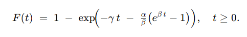
The cumulative distribution function (CDF) is:
The hazard rate is
h(t) = α + β exp [γ t].
When α = 0, the model reduces to the Gompertz model; The Gompertz-Makeham model reduces to the exponential model when γ = 0 [4].
The Gompertz-Makeham distribution has several important properties that make it useful in modeling lifetimes. For one, it is a highly flexible distribution that can fit a wide range of mortality patterns.
Additionally, it has a closed-form solution (i.e., an expression for an exact solution given with a finite amount of data) for its pdf and CDF, which makes it easy to work with mathematically. Finally, it provides a way to estimate life expectancy and other mortality measures, such as the probability of dying within a certain age range.
Gompertz Function
The Gompertz function, the building block for the Gompertz-Makeham distribution as well as many other life distributions [5], is expressed as: Rm = R0 eat, Where:
- Rm = mortality rate,
- a and R0 = constants,
- t = time parameter.
Perks distribution
The Perks distribution, an extension of the Gompertz–Makeham distribution, has many applications in actuarial science and survival analysis including pensioner mortality data [6]. It is named after W. Perks, who proposed the distribution in his 1932 actuarial paper On some experiments in the graduation of mortality statistics [7].
The distribution is seldom seen, perhaps because its parameters are challenging to estimate without advanced methods such as Markov Chain Monte Carlo (MCMC), In addition, its moments are not available in closed form.
Probability density function (PDF):
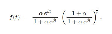
Where
- α is a shape parameter
- β is a scale parameter.
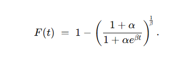
Cumulative distribution function (CDF):
The term “Perks’s distribution” is sometimes used to refer to the distribution of the mean in samples from a population with the form [8]
(2λ) / (π (eλx + e^ – λx)).
Extensions include the four-parameter Kumaraswamy Perks distribution (also called the KumPerks distribution) proposed by Oguntunde [9].
References
Image: NIST. Retrieved November 15, 2021 from: https://www.itl.nist.gov/div898/software/dataplot/refman2/auxillar/makpdf.htm
- Henderson, A. (1968). Actuarial methods for estimating morality parameters of industrial property.
- GompertzMakehamDistribution. Retrieved November 15, 2021 from: https://reference.wolfram.com/language/ref/GompertzMakehamDistribution.html
- Butt, Z. & Haberman, S. Application of Frailty-Based Mortality Models using Generalized Linear Models.
- Leemis. Theorem. Retrieved November 15, 2021 from: http://www.math.wm.edu/~leemis/chart/UDR/PDFs/MakehamGompertz.pdf
- [Gompertz, 1825] as cited in Norström, F. The Gompertz-Makeham distribution. Retrieved November 15, 2021 from: http://citeseerx.ist.psu.edu/viewdoc/download?doi=10.1.1.1068.8330&rep=rep1&type=pdf
- Haberman, S.; Renshaw, A. A comparative study of parametric mortality projection models. Insur. Math. Econ. 2011, 48, 35–55. [Google Scholar]
- Perks W (1932) On some experiments in the graduation of mortality statistics. J Inst Actuar 43:12–57
- Commenges, D. et al. (2003). The Oxford Dictionary of Statistical Terms.
- Ogutunde, P. Introducing the Kumaraswamy Perks Distribution. Proceedings of the World Congress on Engineering and Computer Science 2018 Vol II WCECS 2018, October 23-25, 2018, San Francisco, USA