Probability Distributions > Reciprocal distribution
What is a Reciprocal Distribution?
There isn’t a universal definition for the “reciprocal distribution.” Definitions from the literature include:
- Any distribution of a reciprocal of a random variable [1]).
- A reciprocal continuous random variable [2].
- A synonym for the logarithmic distribution [3].
That said, most probability density functions (pdfs) for a reciprocal distribution involve a logarithm in one form or another: for pink noise, distributions of mantissas (the part of a logarithm that follows the decimal point), or the under-workings of Benford’s law.
At a glance, the most common or historically important applications of the reciprocal distribution are:
- Bayesian Inference: As an uninformative/Jeffreys prior on scale parameters.
- Pink (1/f) Noise: Often modeled via power-law or reciprocal-like distributions for amplitude or power spectra.
- Floating Point and Mantissas: Hamming’s argument that numerical processes produce a log-uniform distribution of mantissas.
- Benford’s Law: Related to the distribution of leading digits, underpinned by scale invariance and the 1/x factor.
- Any Reciprocal Random Variable: In the broadest sense, if = 1/, then “the distribution of ” is sometimes called “the reciprocal distribution of .”
Of all the different versions of the pdf for the reciprocal distribution, the pink noise/Bayesian inference one is by far the most common.
Synonyms for the reciprocal distribution include: log-uniform, 1/x distribution, scale-invariant distribution, and Jeffreys prior for scale. Note that the term “logarithmic distribution” is sometimes (incorrectly) conflated with “log-uniform distribution.”
1. Pink Noise / Bayesian Inference
The reciprocal distribution is used to describe pink (1/f) noise, or as an uninformed prior distribution for scale parameters in Bayesian inference.
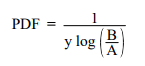
SciPy stats also uses this PDF.
A key reason the reciprocal distribution appears so often—especially in Bayesian inference—is that it is scale-invariant (sometimes called “invariant under scale transformations”) and is the Jeffreys prior for scale parameters. In other words, if X has a reciprocal distribution, then αX has the same “shape” of distribution (up to normalization) for any constant α > 0.
- Jeffreys Prior for a Scale Parameter: If θ is a scale parameter (e.g., standard deviation σ), an uninformative prior for θ is often taken as p(θ) ∝ 1/θ, precisely because it is invariant under re-scaling.
2. Distribution of Mantissas
The mantissa is the part of the logarithm following the decimal point, or the part of the floating point number (closely related to scientific notation) following the decimal point. For example, .12345678 * 102, .12345678 is the mantissa.
In his book, Numerical Methods for Scientists and Engineers, Richard Hamming uses a reciprocal distribution to describe the probability of finding the number x in the base b (The base in logarithmic calculation is the subscript to the right of “log”; the base in log3(x) is “3”). The pdf for this probability is:
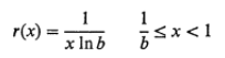
Why do mantissas end up “reciprocally” distributed?
Because floating-point multiplications and divisions essentially redistribute significant digits (“mantissas”) in a way that is uniform in log-space rather than linear-space. This phenomenon underlies the limiting form that emerges in many numerical processes, as well as its relevance to Benford’s law.
3. Reciprocal Distribution (Benford’s Law)
The reciprocal distribution is a continuous probability distribution defined on the open interval (a, b). The Probability Density Function (PDF) is
r(x) ≡ c/x,
Where:
- x = a random variable,
- c = the normalization constant c = 1/ ln b (when x ranges from 1/b to 1).
This PDF is the underpinnings of Benford’s Law [6].
4. Other Uses and Meanings
Outside of probability and statistics, the term “reciprocal distribution” doesn’t involve a probability distribution at all; it refers to You scratch my back and I’ll scratch yours. For example “Reciprocal distribution of raw materials is only fair—”.
Relationship to the Log-Uniform Distribution
In many texts (including SciPy’s documentation), the “reciprocal distribution” is taken to be identical to the log-uniform distribution on [a, b]. That is,
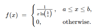
Some authors use the phrase “reciprocal distribution” specifically only for this log-uniform pdf. Others, however, use the phrase in broader or different ways. Here is the main difference between the two uses:
- The logarithmic distribution usually refers to a discrete distribution related to the logarithm series distribution (sometimes used in ecology or species-abundance models).
- The log-uniform (reciprocal) distribution is a continuous distribution with PDF ∝ 1/x.
References
- Marshall, A. & Olkin, L. (2007). Life Distributions: Structure of Nonparametric, Semiparametric, and Parametric Families.
- SciPy Stats (2009). scipy.stats.reciprocal. Retrievd December 11, 2017 from: https://docs.scipy.org/doc/scipy-0.14.0/reference/generated/scipy.stats.reciprocal.html
- Bose, P. & Morin, P. (2003). Algorithms and Computation: 13th International Symposium, ISAAC 2002 Vancouver, BC, Canada, November 21-23, 2002, Proceedings.
- McLaughlin, M. (1999). Regress+: A Compendium of Common Probability Distributions. Retrieved 5/18/23 from http://www.ub.edu/stat/docencia/Diplomatura/Compendium.pdf
- Hamming, R. (2012). Numerical Methods for Scientists and Engineers. Courier Corporation.
- Friar et al., (2016). Ubiquity of Benford’s law and emergence of the reciprocal distribution. Physics Letters A, Volume 380, Issue 22-23, p. 1895-1899.