> List of probability distributions > exponentiated Weibull distribution
What is the exponentiated Weibull distribution?
The exponentiated Weibull distribution (or EW distribution), a generalization of the Weibull distribution, was first proposed by Mudholkar and Srivastava in 1993 [1] as a flexible alternative to the Weibull. It is especially useful when modeling lifetime data with unimodal hazard rates.
The distribution is formed by exponentiating the Weibull cumulative distribution function (CDF); adding a second shape parameter makes the distribution more flexible than the Weibull in terms of the shapes it can accommodate for the hazard rate function. For example, it can handle increasing, decreasing, bathtub-shaped, and unimodal hazard rates. However, this additional flexibility can make it more challenging to estimate model parameters. In addition, the EW distribution may need larger sample sizes than the Weibull to estimate parameters accurately.
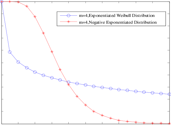
The negative exponential distribution is an alternative for modeling lifetime data; in some cases, the EW distribution can reduce to the negative exponential distribution. However, the EW distribution can accommodate non-monotonic (fluctuating) hazard rates, which the negative exponential cannot.
Exponentiated Weibull distribution properties
The cumulative distribution function (CDF) is:
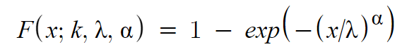
for x > 0, and F(x; k; λ; α) = 0 for x < 0 and
- k > 0 and α > 0 = shape parameters.
- λ > 0 = scale parameter.
The probability density function (pdf) of the EW distribution is given by:

When α = 1, the EW distribution reduces to the Weibull. When k = 1, the pdf gives the exponentiated exponential distribution.
Exponentiated Weibull distribution history and use
Before the introduction of the exponentiated Weibull distribution, many distributions could not accommodate non-monotonic hazard rates, and the existing distributions that could accommodate these hazard rates were not very flexible.
In survival analysis, the hazard rate is defined as the probability an event occurs in a small interval of time, given that the event hasn’t happened yet. For example, when studying machine failure times, the hazard rate would be the instantaneous rate at which the machine is likely to fail at a given time, given that it has not already failed. The graph of a non-monotonic hazard rate has a shape that is not monotonic (i.e., always increasing or always decreasing) but instead tends to vary over time. For example, a bathtub-shaped hazard rate shows a higher hazard rate during its initial phase, followed by a relatively low hazard rate and then another high hazard rate toward the end of the study period.
The EW distribution was first introduced by Mudholkar and Srivastava in 1993 [1], and its flexibility compared to the Weibull distribution was noted. The family of distributions was later extended by different researchers, including Kus et al. [3].
References
- Mudholkar, G. S., & Srivastava, D. K. (1993). Exponentiated Weibull family for analyzing bathtub failure-rate data. IEEE Transactions on Reliability, 42(2), 299-302. https://doi.org/10.1109/24.229504
- Research on Laser Atmospheric Transmission Performance Based on Exponentiated Weibull Distribution Channel Model – Scientific Figure on ResearchGate. Available from: https://www.researchgate.net/figure/Comparison-of-exponentiated-Weibull-distribution-and-negative-exponential-distribution_fig1_289049297 [accessed 9 May, 2023] Creative Commons Attribution 4.0 International
- Kus, C., Unal, G., & Cevik, A. S. (2008). The Exponentiated Weibull Distribution: A Survey. Hacettepe Journal of Mathematics and Statistics, 37(1), 79-91. https://dergipark.org.tr/tr/download/article-file/191632