Exponential Distribution / Negative Exponential: Definition, Examples

< Probability Distributions > Exponential Distribution

Contents:

What is an Exponential Distribution?
What is a Poisson Process?
Uses in real life
Memoryless Property
Exponential PDF
Exponential CDF
Connection to other distributions
Exponential Family
Linear Exponential Distribution

What is an Exponential distribution?

exponential distribution pdf — PDF of the exponential distribution.

The exponential distribution, frequently used in reliability tests, describes time between events in a Poisson process, or time between elapsed events. It is a continuous analog of the geometric distribution [1].

The distribution has a wide range of other applications, including in the Monte Carlo method, where random variables from a rectangular distribution are transformed to exponential random variables. Another application is producing approximate solutions for challenging distributional problems [2].

There is a strong relationship between the Poisson distribution and the Exponential distribution. For example, let’s say a Poisson distribution models the number of births in a given time period. The time in between each birth can be modeled with an exponential distribution [3].

What is a Poisson Process?

The Poisson process gives you a way to find probabilities for random points in time for a process. A “process” could be almost anything:

Accidents at an interchange.
File requests on a server.
Customers arriving at a store.
Battery failure and replacement.

The Poisson process can tell you when one of these random points in time will likely happen. For example, when customers will arrive at a store, or when a battery might need to be replaced. It’s basically a counting process; it counts the number of times an event has occurred since a given point in time, like 1210 customers since 1 p.m., or 543 files since noon.

An assumption for the process is that it is only used for independent events.

Poisson Process Example

Let’s say a store is interested in the number of customers per hour. Arrivals per hour has a Poisson 120 arrival rate, which means that 120 customers arrive per hour. This could also be worded as “The expected mean inter-arrival time is 0.5 minutes”, because a customer can be expected every half minute — 30 seconds.

The negative exponential distribution models this process, so we could write:

Poisson 120 = Exponential 0.5

So the units for the Poisson process are people and the units for the exponential are minutes.

The 120 customers per hour could also be broken down into categories, like men (probability of 0.5), women (probability of 0.3) and children (probability of 0.2). You could calculate the time interval between the arrivals times of women, men, or children.

For example:

The time between arrivals of women would be: A rate 0.3*120 = 36 per hour, or one every 100 seconds.
For men it would be: A rate of 0.5*120 = 60 per hour, or one every minute.
And for children: A rate of 0.2*120 = 24 per hour, or one every 150 seconds.

What is the Exponential Distribution used for?

The exponential distribution is mostly used for testing product reliability. It’s also an important distribution for building continuous-time Markov chains. The exponential often models waiting times and can help you to answer questions like:

“How much time will go by before a major hurricane hits the Atlantic Seaboard?” or
“How long will the transmission in my car last before it breaks?”.

If you assume that the answer to these questions is unknown, you can think of the elapsed time as a random variable with an exponential distribution as long as the events occur continuously and independently at a constant rate.

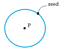
Exponential Distribution - Young and Young chart — The exponential distribution can model area, as well as time, between events.

Young and Young [3] give an example of how the exponential distribution can also model space between events (instead of time between events). Say that grass seeds are randomly dispersed over a field; Each point in the field has an equal chance of a seed landing there. Now select a point P, then measure the distance to the nearest seed. This distance becomes the radius for a circle with point P at the center. The circle’s area has an exponential distribution.

Memoryless Property

This distribution has a memoryless property, which means it “forgets” what has come before it. In other words, if you continue to wait, the length of time you wait neither increases nor decreases the probability of an event happening. Any time may be marked down as time zero.

Let’s say a hurricane hits your island. The probability of another hurricane hitting in one week, one month, or ten years from that point are all equal.

The exponential is the only distribution with the memoryless property. While many authors consider the memoryless property to be one of the most useful aspects of the distribution, it’s also the reason why it may not make sense for modeling certain situations.

For example, let’s say you wanted to model deaths of family dogs. Because of the memoryless property, the probability of a pet dog dying at age 1 would be the same as the dog dying at age 15, which is obviously nonsensical. Therefore, you should think about whether the exponential makes sense logically to your particular area of interest.

For lifetime studies, the exponential is usually used only as a first rough model for the process.

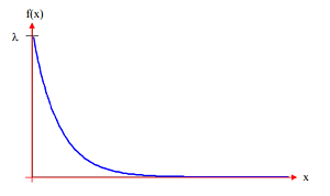
Probability Density Function

The most common form of the pdf is:

F(x;λ) = e^-λx x > 0.

Where:

e = the natural number e,
λ = mean time between events,
x = a random variable.

For x less than 0, F(x;λ) = 0 A variety of other notation is in use. For example, the scale parameter is sometimes also referred to as β, where

β = 1/λ

This process of switching out the two expressions is called reparameterization. One way to think about why we’re using a reciprocal here is to think about what it represents. The reciprocal 1/β is expressed as units of time, while λ is a rate. For example, let’s say you log a sale in your bookstore four times an hour; this is the rate, λ = 4. But you can also express this in units of time: one sale every ¼ of an hour (or 15 minutes). An alternate form of the pdf [4] is:

f(x) = (1/β) e^{− (x − μ) / β} x ≥ μ ; β > 0

where μ is the location parameter and β is the scale parameter.

If μ = 0 and β = 1 it is called the standard exponential distribution and has the equation:

f(x)=e^−x for x ≥ 0.

You might also see the scale parameter as σ.

Cumulative Distribution Function

The formula for the cumulative distribution function of the exponential distribution is:

F(x) = 1 − e^{− λx} x ≥ 0; λ > 0

Connection to Other Distributions

The exponential distribution is related to the Poisson distribution. While the exponential models time between successive events over a continuous time interval, the Poisson distribution deals with events that happen over a fixed period of time. The number of times the event will happen within a certain amount of time is a Poisson distribution if:

The event can happen more than one time.
If the time elapsed between two events is exponentially distributed.
The events are independent of previous events.

Using this definition, some natural events can fit the model. For example, the number of hurricanes that hit Hawaii each year is a Poisson distribution. However, figuring out when a machine might fail is not (as the event can only happen once). The exponential is a special case of the gamma distribution [5]. It is the continuous counterpart of the geometric distribution, which models time between successes in a series of independent trials. The exponential distribution is also a special case of the Weibull distribution, which happens when the Weibull shape parameter = 1.

Linear Exponential Distribution

The linear exponential (LE) distribution is an extension of the exponential distribution. It is often used in actuarial science and survival analysis, where it is sometimes called the linear failure rate distribution. The LE describes survival patterns with constant initial hazard rates. The “linear” part of the distribution is the hazard rate, which varies as a linear function of age or time .

The distribution is one of the best models to fit data that has an increasing failure rate. It is not a good choice for modeling data that has decreasing, non linear increasing, or non-monotone failure rates.

PDF of the Linear Exponential Distribution

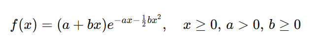
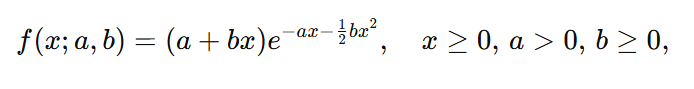
If you begin with an exponential distribution with a constant failure rate

f(x) = a + bx,

the result is the linear exponential distribution with a distribution function of

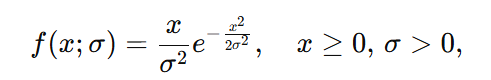
There are, however, a wide range of members in the linear exponential family, so you’ll come across a wide variety of different pdfs, which range from the basic to the complex. For example, the Rayleigh distribution — a submodel of the LE — has PDF

At the other end of the spectrum, the Tweedie distribution — a member of the linear exponential family of distributions, has a pdf that is complex and cannot be expressed in closed form; it’s sometimes expressed as a series of functions.

A two parameter PDF of the linear exponential distribution can be described by

For more details on how the different types are defined, see linear exponential family.

Exponential Family

The exponential distribution is one member of a very large class of probability distributions called the exponential families, or exponential classes. Some of the more well-known members of this family include:

The Bernoulli distribution,
The beta distribution,
The binomial distribution (for a fixed number of trials),
The Categorical distribution,
The Chi-squared distribution,
The Dirichlet distribution,
The gamma distribution,
The Geometric distribution,
The inverse Gaussian distribution,
The lognormal distribution.
The negative binomial distribution (for a fixed number of failures),
The normal distribution,
Poisson distribution
The von-Mises distribution,
The von-Mises Fisher distribution.

This vast variety of distributions are connected in that they all have the following general form for their density (relative to their parameter vector, η):

References

- Lee, E. & Wang, J. (2003). Statistical Methods for Survival Data Analysis. Wiley.
- El-Damcese, M. & Marei, Gh. (2012). Extension of the Linear Exponential Distribution and its Applications. International Journal of Science and Research (IJSR). ISSN (Online): 2319-7064.
- Young & Young (1998). Statistical Ecology. Springer Science and Business Media.
- Engineering Statistics Handbook (n.d.). Exponential Dist. Retrieved October 22, 2017 from: http://www.itl.nist.gov/div898/handbook/eda/section3/eda3667.htm.
- Balakrishnan, K. (1996). Exponential Dist: Theory, Methods and Applications. CRC Press.